Geospatial data is data about specific locations on the earth’s surface. It can represent a geographical area as a whole or it can represent an event associated with a geographical area. Analysis of geospatial data is sought after in a few industries. It involves understanding where the data exists from a spatial perspective and why it exists there.
There are two types of geospatial data: vector data and raster data. Raster data is a matrix of cells represented as a grid, mostly representing photographs and satellite imagery. In this post, we focus on vector data, which is represented as geographical coordinates of latitude and longitude as well as lines and polygons (areas) connecting or encompassing them. Vector data has a multitude of use cases in deriving mobility insights. User mobile data is one such component of it, and it’s derived mostly from the geographical position of mobile devices using GPS or app publishers using SDKs or similar integrations. For the purpose of this post, we refer to this data as mobility data.
This is a two-part series. In this first post, we introduce mobility data, its sources, and a typical schema of this data. We then discuss the various use cases and explore how you can use AWS services to clean the data, how machine learning (ML) can aid in this effort, and how you can make ethical use of the data in generating visuals and insights. The second post will be more technical in nature and cover these steps in detail alongside sample code. This post does not have a sample dataset or sample code, rather it covers how to use the data after it’s purchased from a data aggregator.
You can use Amazon SageMaker geospatial capabilities to overlay mobility data on a base map and provide layered visualization to make collaboration easier. The GPU-powered interactive visualizer and Python notebooks provide a seamless way to explore millions of data points in a single window and share insights and results.
Sources and schema
There are few sources of mobility data. Apart from GPS pings and app publishers, other sources are used to augment the dataset, such as Wi-Fi access points, bid stream data obtained via serving ads on mobile devices, and specific hardware transmitters placed by businesses (for example, in physical stores). It’s often difficult for businesses to collect this data themselves, so they may purchase it from data aggregators. Data aggregators collect mobility data from various sources, clean it, add noise, and make the data available on a daily basis for specific geographic regions. Due to the nature of the data itself and because it’s difficult to obtain, the accuracy and quality of this data can vary considerably, and it’s up to the businesses to appraise and verify this by using metrics such as daily active users, total daily pings, and average daily pings per device. The following table shows what a typical schema of a daily data feed sent by data aggregators may look like.
| Attribute | Description |
| Id or MAID | Mobile Advertising ID (MAID) of the device (hashed) |
| lat | Latitude of the device |
| lng | Longitude of the device |
| geohash | Geohash location of the device |
| device_type | Operating System of the device = IDFA or GAID |
| horizontal_accuracy | Accuracy of horizontal GPS coordinates (in meters) |
| timestamp | Timestamp of the event |
| ip | IP address |
| alt | Altitude of the device (in meters) |
| speed | Speed of the device (in meters/second) |
| country | ISO two-digit code for the country of origin |
| state | Codes representing state |
| city | Codes representing city |
| zipcode | Zipcode of where Device ID is seen |
| carrier | Carrier of the device |
| device_manufacturer | Manufacturer of the device |
Use cases
Mobility data has widespread applications in varied industries. The following are some of the most common use cases:
- Density metrics – Foot traffic analysis can be combined with population density to observe activities and visits to points of interest (POIs). These metrics present a picture of how many devices or users are actively stopping and engaging with a business, which can be further used for site selection or even analyzing movement patterns around an event (for example, people traveling for a game day). To obtain such insights, the incoming raw data goes through an extract, transform, and load (ETL) process to identify activities or engagements from the continuous stream of device location pings. We can analyze activities by identifying stops made by the user or mobile device by clustering pings using ML models in Amazon SageMaker.
- Trips and trajectories – A device’s daily location feed can be expressed as a collection of activities (stops) and trips (movement). A pair of activities can represent a trip between them, and tracing the trip by the moving device in geographical space can lead to mapping the actual trajectory. Trajectory patterns of user movements can lead to interesting insights such as traffic patterns, fuel consumption, city planning, and more. It can also provide data to analyze the route taken from advertising points such as a billboard, identify the most efficient delivery routes to optimize supply chain operations, or analyze evacuation routes in natural disasters (for example, hurricane evacuation).
- Catchment area analysis – A catchment area refers to places from where a given area draws its visitors, who may be customers or potential customers. Retail businesses can use this information to determine the optimal location to open a new store, or determine if two store locations are too close to each other with overlapping catchment areas and are hampering each other’s business. They can also find out where the actual customers are coming from, identify potential customers who pass by the area traveling to work or home, analyze similar visitation metrics for competitors, and more. Marketing Tech (MarTech) and Advertisement Tech (AdTech) companies can also use this analysis to optimize marketing campaigns by identifying the audience close to a brand’s store or to rank stores by performance for out-of-home advertising.
There are several other use cases, including generating location intelligence for commercial real estate, augmenting satellite imagery data with footfall numbers, identifying delivery hubs for restaurants, determining neighborhood evacuation likelihood, discovering people movement patterns during a pandemic, and more.
Challenges and ethical use
Ethical use of mobility data can lead to many interesting insights that can help organizations improve their operations, perform effective marketing, or even attain a competitive advantage. To utilize this data ethically, several steps need to be followed.
It starts with the collection of data itself. Although most mobility data remains free of personally identifiable information (PII) such as name and address, data collectors and aggregators must have the user’s consent to collect, use, store, and share their data. Data privacy laws such as GDPR and CCPA need to be adhered to because they empower users to determine how businesses can use their data. This first step is a substantial move towards ethical and responsible use of mobility data, but more can be done.
Each device is assigned a hashed Mobile Advertising ID (MAID), which is used to anchor the individual pings. This can be further obfuscated by using Amazon Macie, Amazon S3 Object Lambda, Amazon Comprehend, or even the AWS Glue Studio Detect PII transform. For more information, refer to Common techniques to detect PHI and PII data using AWS Services.
Apart from PII, considerations should be made to mask the user’s home location as well as other sensitive locations like military bases or places of worship.
The final step for ethical use is to derive and export only aggregated metrics out of Amazon SageMaker. This means getting metrics such as average number or total number of visitors as opposed to individual travel patterns; getting daily, weekly, monthly or yearly trends; or indexing mobility patters over publicly available data such as census data.
Solution overview
As mentioned earlier, the AWS services that you can use for analysis of mobility data are Amazon S3, Amazon Macie, AWS Glue, S3 Object Lambda, Amazon Comprehend, and Amazon SageMaker geospatial capabilities. Amazon SageMaker geospatial capabilities make it easy for data scientists and ML engineers to build, train, and deploy models using geospatial data. You can efficiently transform or enrich large-scale geospatial datasets, accelerate model building with pre-trained ML models, and explore model predictions and geospatial data on an interactive map using 3D accelerated graphics and built-in visualization tools.
The following reference architecture depicts a workflow using ML with geospatial data.
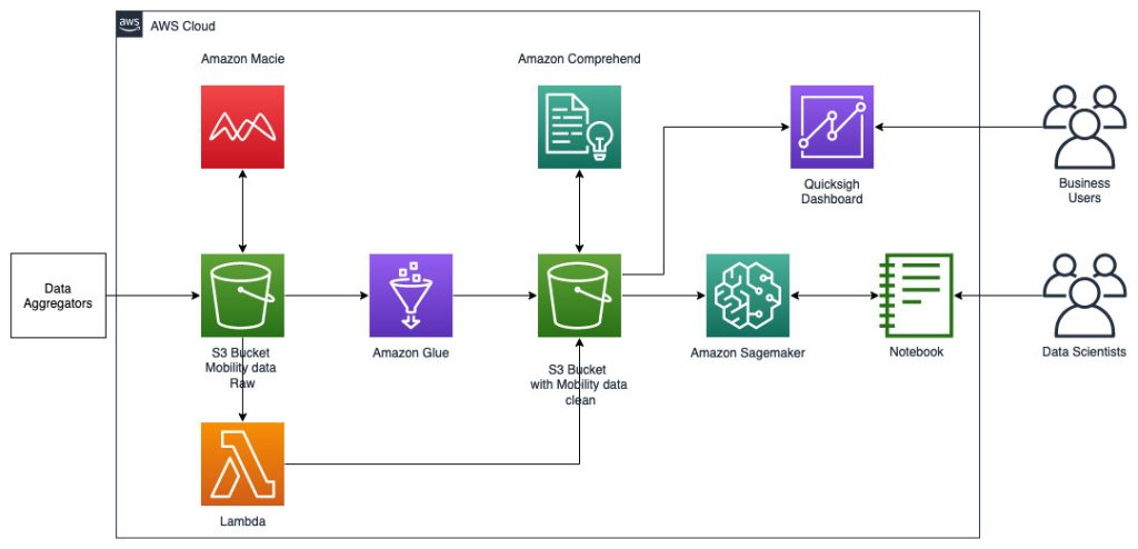
In this workflow, raw data is aggregated from various data sources and stored in an Amazon Simple Storage Service (S3) bucket. Amazon Macie is used on this S3 bucket to identify and redact and PII. AWS Glue is then used to clean and transform the raw data to the required format, then the modified and cleaned data is stored in a separate S3 bucket. For those data transformations that are not possible via AWS Glue, you use AWS Lambda to modify and clean the raw data. When the data is cleaned, you can use Amazon SageMaker to build, train, and deploy ML models on the prepped geospatial data. You can also use the geospatial Processing jobs feature of Amazon SageMaker geospatial capabilities to preprocess the data—for example, using a Python function and SQL statements to identify activities from the raw mobility data. Data scientists can accomplish this process by connecting through Amazon SageMaker notebooks. You can also use Amazon QuickSight to visualize business outcomes and other important metrics from the data.
Amazon SageMaker geospatial capabilities and geospatial Processing jobs
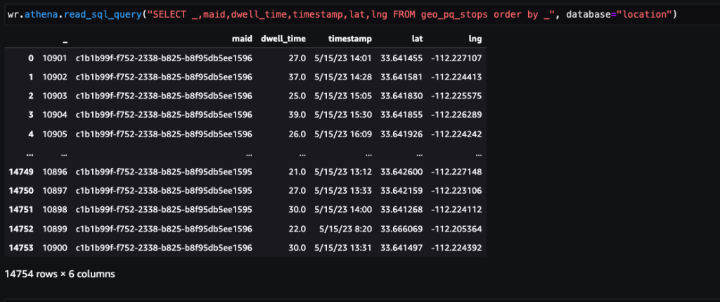
After the data is obtained and fed into Amazon S3 with a daily feed and cleaned for any sensitive data, it can be imported into Amazon SageMaker using an Amazon SageMaker Studio notebook with a geospatial image. The following screenshot shows a sample of daily device pings uploaded into Amazon S3 as a CSV file and then loaded in a pandas data frame. The Amazon SageMaker Studio notebook with geospatial image comes preloaded with geospatial libraries such as GDAL, GeoPandas, Fiona, and Shapely, and makes it straightforward to process and analyze this data.

This sample dataset contains approximately 400,000 daily device pings from 5,000 devices from 14,000 unique places recorded from users visiting the Arrowhead Mall, a popular shopping mall complex in Phoenix, Arizona, on May 15, 2023. The preceding screenshot shows a subset of columns in the data schema. The MAID column represents the device ID, and each MAID generates pings every minute relaying the latitude and longitude of the device, recorded in the sample file as Lat and Lng columns.
The following are screenshots from the map visualization tool of Amazon SageMaker geospatial capabilities powered by Foursquare Studio, depicting the layout of pings from devices visiting the mall between 7:00 AM and 6:00 PM.
The following screenshot shows pings from the mall and surrounding areas.

The following shows pings from inside various stores in the mall.

Each dot in the screenshots depicts a ping from a given device at a given point in time. A cluster of pings represents popular spots where devices gathered or stopped, such as stores or restaurants.
As part of the initial ETL, this raw data can be loaded onto tables using AWS Glue. You can create an AWS Glue crawler to identify the schema of the data and form tables by pointing to the raw data location in Amazon S3 as the data source.


As mentioned above, the raw data (the daily device pings), even after initial ETL, will represent a continuous stream of GPS pings indicating device locations. To extract actionable insights from this data, we need to identify stops and trips (trajectories). This can be achieved using the geospatial Processing jobs feature of SageMaker geospatial capabilities. Amazon SageMaker Processing uses a simplified, managed experience on SageMaker to run data processing workloads with the purpose-built geospatial container. The underlying infrastructure for a SageMaker Processing job is fully managed by SageMaker. This feature enables custom code to run on geospatial data stored on Amazon S3 by running a geospatial ML container on a SageMaker Processing job. You can run custom operations on open or private geospatial data by writing custom code with open source libraries, and run the operation at scale using SageMaker Processing jobs. The container-based approach solves for needs around standardization of development environment with commonly used open source libraries.
To run such large-scale workloads, you need a flexible compute cluster that can scale from tens of instances to process a city block, to thousands of instances for planetary-scale processing. Manually managing a DIY compute cluster is slow and expensive. This feature is particularly helpful when the mobility dataset involves more than a few cities to multiple states or even countries and can be used to run a two-step ML approach.
The first step is to use density-based spatial clustering of applications with noise (DBSCAN) algorithm to cluster stops from pings. The next step is to use the support vector machines (SVMs) method to further improve the accuracy of the identified stops and also to distinguish stops with engagements with a POI vs. stops without one (such as home or work). You can also use SageMaker Processing job to generate trips and trajectories from the daily device pings by identifying consecutive stops and mapping the path between the source and destinations stops.
After processing the raw data (daily device pings) at scale with geospatial Processing jobs, the new dataset called stops should have the following schema.
| Attribute | Description |
| Id or MAID | Mobile Advertising ID of the device (hashed) |
| lat | Latitude of the centroid of the stop cluster |
| lng | Longitude of the centroid of the stop cluster |
| geohash | Geohash location of the POI |
| device_type | Operating system of the device (IDFA or GAID) |
| timestamp | Start time of the stop |
| dwell_time | Dwell time of the stop (in seconds) |
| ip | IP address |
| alt | Altitude of the device (in meters) |
| country | ISO two-digit code for the country of origin |
| state | Codes representing state |
| city | Codes representing city |
| zipcode | Zip code of where device ID is seen |
| carrier | Carrier of the device |
| device_manufacturer | Manufacturer of the device |
Stops are consolidated by clustering the pings per device. Density-based clustering is combined with parameters such as the stop threshold being 300 seconds and the minimum distance between stops being 50 meters. These parameters can be adjusted as per your use case.
The following screenshot shows approximately 15,000 stops identified from 400,000 pings. A subset of the preceding schema is present as well, where the column Dwell Time represents the stop duration, and the Lat and Lng columns represent the latitude and longitude of the centroids of the stops cluster per device per location.
Post-ETL, data is stored in Parquet file format, which is a columnar storage format that makes it easier to process large amounts of data.

The following screenshot shows the stops consolidated from pings per device inside the mall and surrounding areas.

After identifying stops, this dataset can be joined with publicly available POI data or custom POI data specific to the use case to identify activities, such as engagement with brands.
The following screenshot shows the stops identified at major POIs (stores and brands) inside the Arrowhead Mall.

Home zip codes have been used to mask each visitor’s home location to maintain privacy in case that is part of their trip in the dataset. The latitude and longitude in such cases are the respective coordinates of the centroid of the zip code.
The following screenshot is a visual representation of such activities. The left image maps the stops to the stores, and the right image gives an idea of the layout of the mall itself.

This resulting dataset can be visualized in a number of ways, which we discuss in the following sections.
Density metrics
We can calculate and visualize the density of activities and visits.
Example 1 – The following screenshot shows top 15 visited stores in the mall.

Example 2 – The following screenshot shows number of visits to the Apple Store by each hour.

Trips and trajectories
As mentioned earlier, a pair of consecutive activities represents a trip. We can use the following approach to derive trips from the activities data. Here, window functions are used with SQL to generate the trips table, as shown in the screenshot.


After the trips table is generated, trips to a POI can be determined.
Example 1 – The following screenshot shows the top 10 stores that direct foot traffic towards the Apple Store.

Example 2 – The following screenshot shows all the trips to the Arrowhead Mall.

Example 3 – The following video shows the movement patterns inside the mall.
Example 4 – The following video shows the movement patterns outside the mall.

Catchment area analysis
We can analyze all visits to a POI and determine the catchment area.
Example 1 – The following screenshot shows all visits to the Macy’s store.

Example 2 – The following screenshot shows the top 10 home area zip codes (boundaries highlighted) from where the visits occurred.

Data quality check
We can check the daily incoming data feed for quality and detect anomalies using QuickSight dashboards and data analyses. The following screenshot shows an example dashboard.

Conclusion
Mobility data and its analysis for gaining customer insights and obtaining competitive advantage remains a niche area because it’s difficult to obtain a consistent and accurate dataset. However, this data can help organizations add context to existing analysis and even produce new insights around customer movement patterns. Amazon SageMaker geospatial capabilities and geospatial Processing jobs can help implement these use cases and derive insights in an intuitive and accessible way.
In this post, we demonstrated how to use AWS services to clean the mobility data and then use Amazon SageMaker geospatial capabilities to generate derivative datasets such as stops, activities, and trips using ML models. Then we used the derivative datasets to visualize movement patterns and generate insights.
You can get started with Amazon SageMaker geospatial capabilities in two ways:
To learn more, visit Amazon SageMaker geospatial capabilities and Getting Started with Amazon SageMaker geospatial. Also, visit our GitHub repo, which has several example notebooks on Amazon SageMaker geospatial capabilities.
About the Authors
 Jimy Matthews is an AWS Solutions Architect, with expertise in AI/ML tech. Jimy is based out of Boston and works with enterprise customers as they transform their business by adopting the cloud and helps them build efficient and sustainable solutions. He is passionate about his family, cars and Mixed martial arts.
 Girish Keshav is a Solutions Architect at AWS, helping out customers in their cloud migration journey to modernize and run workloads securely and efficiently. He works with leaders of technology teams to guide them on application security, machine learning, cost optimization and sustainability. He is based out of San Francisco, and loves traveling, hiking, watching sports, and exploring craft breweries.
 Ramesh Jetty is a Senior leader of Solutions Architecture focused on helping AWS enterprise customers monetize their data assets. He advises executives and engineers to design and build highly scalable, reliable, and cost effective cloud solutions, especially focused on machine learning, data and analytics. In his free time he enjoys the great outdoors, biking and hiking with his family.
- SEO Powered Content & PR Distribution. Get Amplified Today.
- PlatoData.Network Vertical Generative Ai. Empower Yourself. Access Here.
- PlatoAiStream. Web3 Intelligence. Knowledge Amplified. Access Here.
- PlatoESG. Carbon, CleanTech, Energy, Environment, Solar, Waste Management. Access Here.
- PlatoHealth. Biotech and Clinical Trials Intelligence. Access Here.
- Source: https://aws.amazon.com/blogs/machine-learning/use-mobility-data-to-derive-insights-using-amazon-sagemaker-geospatial-capabilities/