Efficient control policies enable industrial companies to increase their profitability by maximizing productivity while reducing unscheduled downtime and energy consumption. Finding optimal control policies is a complex task because physical systems, such as chemical reactors and wind turbines, are often hard to model and because drift in process dynamics can cause performance to deteriorate over time. Offline reinforcement learning is a control strategy that allows industrial companies to build control policies entirely from historical data without the need for an explicit process model. This approach does not require interaction with the process directly in an exploration stage, which removes one of the barriers for the adoption of reinforcement learning in safety-critical applications. In this post, we will build an end-to-end solution to find optimal control policies using only historical data on Amazon SageMaker using Ray’s RLlib library. To learn more about reinforcement learning, see Use Reinforcement Learning with Amazon SageMaker.
Use cases
Industrial control involves the management of complex systems, such as manufacturing lines, energy grids, and chemical plants, to ensure efficient and reliable operation. Many traditional control strategies are based on predefined rules and models, which often require manual optimization. It is standard practice in some industries to monitor performance and adjust the control policy when, for example, equipment starts to degrade or environmental conditions change. Retuning can take weeks and may require injecting external excitations in the system to record its response in a trial-and-error approach.
Reinforcement learning has emerged as a new paradigm in process control to learn optimal control policies through interacting with the environment. This process requires breaking down data into three categories: 1) measurements available from the physical system, 2) the set of actions that can be taken upon the system, and 3) a numerical metric (reward) of equipment performance. A policy is trained to find the action, at a given observation, that is likely to produce the highest future rewards.
In offline reinforcement learning, one can train a policy on historical data before deploying it into production. The algorithm trained in this blog post is called “Conservative Q Learning” (CQL). CQL contains an “actor” model and a “critic” model and is designed to conservatively predict its own performance after taking a recommended action. In this post, the process is demonstrated with an illustrative cart-pole control problem. The goal is to train an agent to balance a pole on a cart while simultaneously moving the cart towards a designated goal location. The training procedure uses the offline data, allowing the agent to learn from preexisting information. This cart-pole case study demonstrates the training process and its effectiveness in potential real-world applications.
Solution overview
The solution presented in this post automates the deployment of an end-to-end workflow for offline reinforcement learning with historical data. The following diagram describes the architecture used in this workflow. Measurement data is produced at the edge by a piece of industrial equipment (here simulated by an AWS Lambda function). The data is put into an Amazon Kinesis Data Firehose, which stores it in Amazon Simple Storage Service (Amazon S3). Amazon S3 is a durable, performant, and low-cost storage solution that allows you to serve large volumes of data to a machine learning training process.
AWS Glue catalogs the data and makes it queryable using Amazon Athena. Athena transforms the measurement data into a form that a reinforcement learning algorithm can ingest and then unloads it back into Amazon S3. Amazon SageMaker loads this data into a training job and produces a trained model. SageMaker then serves that model in a SageMaker endpoint. The industrial equipment can then query that endpoint to receive action recommendations.
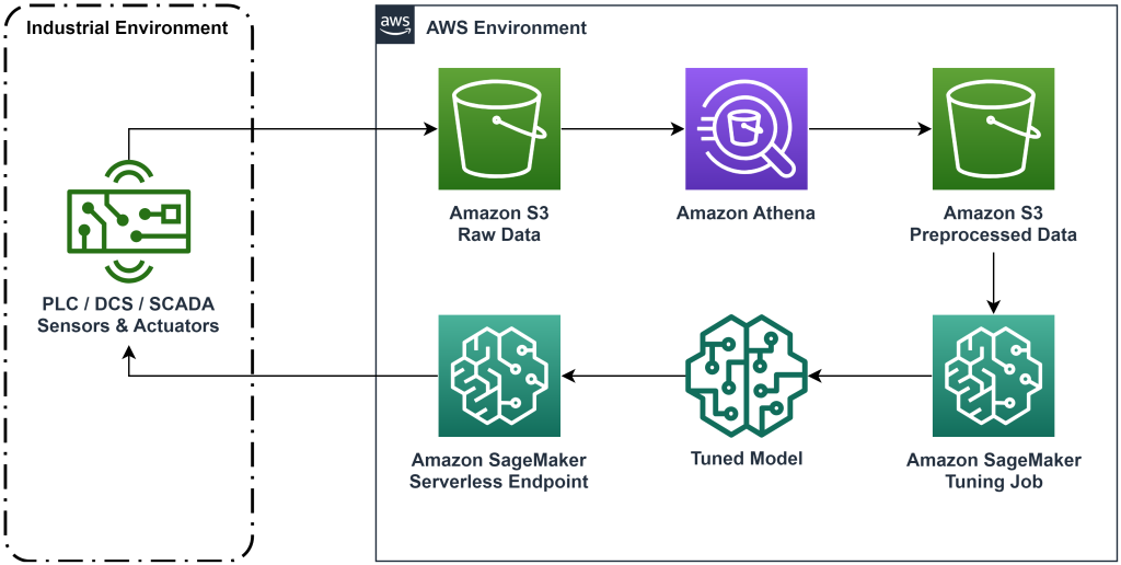
Figure 1: Architecture diagram showing the end-to-end reinforcement learning workflow.
In this post, we will break down the workflow in the following steps:
- Formulate the problem. Decide which actions can be taken, which measurements to make recommendations based on, and determine numerically how well each action performed.
- Prepare the data. Transform the measurements table into a format the machine learning algorithm can consume.
- Train the algorithm on that data.
- Select the best training run based on training metrics.
- Deploy the model to a SageMaker endpoint.
- Evaluate the performance of the model in production.
Prerequisites
To complete this walkthrough, you need to have an AWS account and a command line interface with AWS SAM installed. Follow these steps to deploy the AWS SAM template to run this workflow and generate training data:
- Download the code repository with the command
- Change directory to the repo:
- Build the repo:
- Deploy the repo
- Use the following commands to call a bash script, which generates mock data using an AWS Lambda function.
sudo yum install jqcd utilssh generate_mock_data.sh
Solution walkthrough
Formulate problem
Our system in this blog post is a cart with a pole balanced on top. The system performs well when the pole is upright, and the cart position is close to the goal position. In the prerequisite step, we generated historical data from this system.
The following table shows historical data gathered from the system.
| Cart position | Cart velocity | Pole angle | Pole angular velocity | Goal position | External force | Reward | Time |
| 0.53 | -0.79 | -0.08 | 0.16 | 0.50 | -0.04 | 11.5 | 5:37:54 PM |
| 0.51 | -0.82 | -0.07 | 0.17 | 0.50 | -0.04 | 11.9 | 5:37:55 PM |
| 0.50 | -0.84 | -0.07 | 0.18 | 0.50 | -0.03 | 12.2 | 5:37:56 PM |
| 0.48 | -0.85 | -0.07 | 0.18 | 0.50 | -0.03 | 10.5 | 5:37:57 PM |
| 0.46 | -0.87 | -0.06 | 0.19 | 0.50 | -0.03 | 10.3 | 5:37:58 PM |
You can query historical system information using Amazon Athena with the following query:
The state of this system is defined by the cart position, cart velocity, pole angle, pole angular velocity, and goal position. The action taken at each time step is the external force applied to the cart. The simulated environment outputs a reward value that is higher when the cart is closer to the goal position and the pole is more upright.
Prepare data
To present the system information to the reinforcement learning model, transform it into JSON objects with keys that categorize values into the state (also called observation), action, and reward categories. Store these objects in Amazon S3. Here’s an example of JSON objects produced from time steps in the previous table.
|
{“obs”:[[0.53,-0.79,-0.08,0.16,0.5]], “action”:[[-0.04]], “reward”:[11.5] ,”next_obs”:[[0.51,-0.82,-0.07,0.17,0.5]]} |
|
{“obs”:[[0.51,-0.82,-0.07,0.17,0.5]], “action”:[[-0.04]], “reward”:[11.9], “next_obs”:[[0.50,-0.84,-0.07,0.18,0.5]]} |
|
{“obs”:[[0.50,-0.84,-0.07,0.18,0.5]], “action”:[[-0.03]], “reward”:[12.2], “next_obs”:[[0.48,-0.85,-0.07,0.18,0.5]]} |
The AWS CloudFormation stack contains an output called AthenaQueryToCreateJsonFormatedData. Run this query in Amazon Athena to perform the transformation and store the JSON objects in Amazon S3. The reinforcement learning algorithm uses the structure of these JSON objects to understand which values to base recommendations on and the outcome of taking actions in the historical data.
Train agent
Now we can start a training job to produce a trained action recommendation model. Amazon SageMaker lets you quickly launch multiple training jobs to see how various configurations affect the resulting trained model. Call the Lambda function named TuningJobLauncherFunction to start a hyperparameter tuning job that experiments with four different sets of hyperparameters when training the algorithm.
Select best training run
To find which of the training jobs produced the best model, examine loss curves produced during training. CQL’s critic model estimates the actor’s performance (called a Q value) after taking a recommended action. Part of the critic’s loss function includes the temporal difference error. This metric measures the critic’s Q value accuracy. Look for training runs with a high mean Q value and a low temporal difference error. This paper, A Workflow for Offline Model-Free Robotic Reinforcement Learning, details how to select the best training run. The code repository has a file, /utils/investigate_training.py, that creates a plotly html figure describing the latest training job. Run this file and use the output to pick the best training run.
We can use the mean Q value to predict the performance of the trained model. The Q values are trained to conservatively predict the sum of discounted future reward values. For long-running processes, we can convert this number to an exponentially weighted average by multiplying the Q value by (1-“discount rate”). The best training run in this set achieved a mean Q value of 539. Our discount rate is 0.99, so the model is predicting at least 5.39 average reward per time step. You can compare this value to historical system performance for an indication of if the new model will outperform the historical control policy. In this experiment, the historical data’s average reward per time step was 4.3, so the CQL model is predicting 25 percent better performance than the system achieved historically.
Deploy model
Amazon SageMaker endpoints let you serve machine learning models in several different ways to meet a variety of use cases. In this post, we’ll use the serverless endpoint type so that our endpoint automatically scales with demand, and we only pay for compute usage when the endpoint is generating an inference. To deploy a serverless endpoint, include a ProductionVariantServerlessConfig in the production variant of the SageMaker endpoint configuration. The following code snippet shows how the serverless endpoint in this example is deployed using the Amazon SageMaker software development kit for Python. Find the sample code used to deploy the model at sagemaker-offline-reinforcement-learning-ray-cql.
The trained model files are located at the S3 model artifacts for each training run. To deploy the machine learning model, locate the model files of the best training run, and call the Lambda function named “ModelDeployerFunction” with an event that contains this model data. The Lambda function will launch a SageMaker serverless endpoint to serve the trained model. Sample event to use when calling the “ModelDeployerFunction”:
Evaluate trained model performance
It’s time to see how our trained model is doing in production! To check the performance of the new model, call the Lambda function named “RunPhysicsSimulationFunction” with the SageMaker endpoint name in the event. This will run the simulation using the actions recommended by the endpoint. Sample event to use when calling the RunPhysicsSimulatorFunction:
Use the following Athena query to compare the performance of the trained model with historical system performance.
| Action source | Average reward per time step |
trained_model |
10.8 |
historic_data |
4.3 |
The following animations show the difference between a sample episode from the training data and an episode where the trained model was used to pick which action to take. In the animations, the blue box is the cart, the blue line is the pole, and the green rectangle is the goal location. The red arrow shows the force applied to the cart at each time step. The red arrow in the training data jumps back and forth quite a bit because the data was generated using 50 percent expert actions and 50 percent random actions. The trained model learned a control policy that moves the cart quickly to the goal position, while maintaining stability, entirely from observing nonexpert demonstrations.
 |
 |
Clean up
To delete resources used in this workflow, navigate to the resources section of the Amazon CloudFormation stack and delete the S3 buckets and IAM roles. Then delete the CloudFormation stack itself.
Conclusion
Offline reinforcement learning can help industrial companies automate the search for optimal policies without compromising safety by using historical data. To implement this approach in your operations, start by identifying the measurements that make up a state-determined system, the actions you can control, and metrics that indicate desired performance. Then, access this GitHub repository for the implementation of an automatic end-to-end solution using Ray and Amazon SageMaker.
The post just scratches the surface of what you can do with Amazon SageMaker RL. Give it a try, and please send us feedback, either in the Amazon SageMaker discussion forum or through your usual AWS contacts.
About the Authors
 Walt Mayfield is a Solutions Architect at AWS and helps energy companies operate more safely and efficiently. Before joining AWS, Walt worked as an Operations Engineer for Hilcorp Energy Company. He likes to garden and fly fish in his spare time.
 Felipe Lopez is a Senior Solutions Architect at AWS with a concentration in Oil & Gas Production Operations. Prior to joining AWS, Felipe worked with GE Digital and Schlumberger, where he focused on modeling and optimization products for industrial applications.
 Yingwei Yu is an Applied Scientist at Generative AI Incubator, AWS. He has experience working with several organizations across industries on various proofs of concept in machine learning, including natural language processing, time series analysis, and predictive maintenance. In his spare time, he enjoys swimming, painting, hiking, and spending time with family and friends.
 Haozhu Wang is a research scientist in Amazon Bedrock focusing on building Amazon’s Titan foundation models. Previously he worked in Amazon ML Solutions Lab as a co-lead of the Reinforcement Learning Vertical and helped customers build advanced ML solutions with the latest research on reinforcement learning, natural language processing, and graph learning. Haozhu received his PhD in Electrical and Computer Engineering from the University of Michigan.
- SEO Powered Content & PR Distribution. Get Amplified Today.
- PlatoData.Network Vertical Generative Ai. Empower Yourself. Access Here.
- PlatoAiStream. Web3 Intelligence. Knowledge Amplified. Access Here.
- PlatoESG. Automotive / EVs, Carbon, CleanTech, Energy, Environment, Solar, Waste Management. Access Here.
- PlatoHealth. Biotech and Clinical Trials Intelligence. Access Here.
- ChartPrime. Elevate your Trading Game with ChartPrime. Access Here.
- BlockOffsets. Modernizing Environmental Offset Ownership. Access Here.
- Source: https://aws.amazon.com/blogs/machine-learning/optimize-equipment-performance-with-historical-data-ray-and-amazon-sagemaker/