This post is written in collaboration with Brad Duncan, Rachel Johnson and Richard Alcock from MathWorks.
MATLAB is a popular programming tool for a wide range of applications, such as data processing, parallel computing, automation, simulation, machine learning, and artificial intelligence. It’s heavily used in many industries such as automotive, aerospace, communication, and manufacturing. In recent years, MathWorks has brought many product offerings into the cloud, especially on Amazon Web Services (AWS). For more details about MathWorks cloud products, see MATLAB and Simulink in the Cloud or email Mathworks.
In this post, we bring MATLAB’s machine learning capabilities into Amazon SageMaker, which has several significant benefits:
- Compute resources: Using the high-performance computing environment offered by SageMaker can speed up machine learning training.
- Collaboration: MATLAB and SageMaker together provide a robust platform that t teams can use to collaborate effectively on building, testing, and deploying machine learning models.
- Deployment and accessibility: Models can be deployed as SageMaker real-time endpoints, making them readily accessible for other applications to process live streaming data.
We show you how to train a MATLAB machine learning model as a SageMaker training job and then deploy the model as a SageMaker real-time endpoint so it can process live, streaming data.
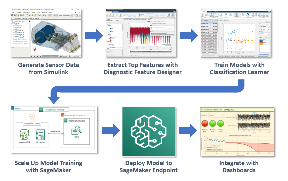
To do this, we’ll use a predictive maintenance example where we classify faults in an operational pump that’s streaming live sensor data. We have access to a large repository of labeled data generated from a Simulink simulation that has three possible fault types in various possible combinations (for example, one healthy and seven faulty states). Because we have a model of the system and faults are rare in operation, we can take advantage of simulated data to train our algorithm. The model can be tuned to match operational data from our real pump using parameter estimation techniques in MATLAB and Simulink.

Our objective is to demonstrate the combined power of MATLAB and Amazon SageMaker using this fault classification example.
We start by training a classifier model on our desktop with MATLAB. First, we extract features from a subset of the full dataset using the Diagnostic Feature Designer app, and then run the model training locally with a MATLAB decision tree model. Once we’re satisfied with the parameter settings, we can generate a MATLAB function and send the job along with the dataset to SageMaker. This allows us to scale up the training process to accommodate much larger datasets. After training our model, we deploy it as a live endpoint which can be integrated into a downstream app or dashboard, such as a MATLAB Web App.
This example will summarize each step, providing a practical understanding of how to leverage MATLAB and Amazon SageMaker for machine learning tasks. The full code and description for the example is available in this repository.
Prerequisites
- Working environment of MATLAB 2023a or later with MATLAB Compiler and the Statistics and Machine Learning Toolbox on Linux. Here is a quick guide on how to run MATLAB on AWS.
- Docker set up in an Amazon Elastic Compute Cloud (Amazon EC2) instance where MATLAB is running. Either Ubuntu or Linux.
- Installation of AWS Command-Line Interface (AWS CLI), AWS Configure, and Python3.
- AWS CLI, should be already installed if you followed the installation guide from step 1.
- Set up AWS Configure to interact with AWS resources.
- Verify your python3 installation by running
python -Vorpython --versioncommand on your terminal. Install Python if necessary.
- Copy this repo to a folder in your Linux machine by running:
- Check the permission on the repo folder. If it does not have write permission, run the following shell command:
- Build the MATLAB training container and push it to the Amazon Elastic Container Registry (Amazon ECR).
- Navigate to folder
docker - Create an Amazon ECR repo using the AWS CLI (replace REGION with your preferred AWS region)
- Run the following docker command:
- Navigate to folder
- Open MATLAB and open the live script called
PumpFaultClassificationMATLABSageMaker.mlxin folderexamples/PumpFaultClassification. Make this folder your current working folder in MATLAB.
Part 1: Data preparation & feature extraction
The first step in any machine learning project is to prepare your data. MATLAB provides a wide range of tools for importing, cleaning, and extracting features from your data.:
The SensorData.mat dataset contains 240 records. Each record has two timetables: flow and pressure. The target column is faultcode, which is a binary representation of three possible fault combinations in the pump. For those time series tables, each table has 1,201 rows which mimic 1.2 seconds of pump flow and pressure measurement with 0.001 seconds increment.

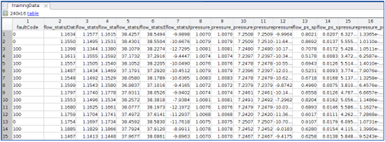
Next, the Diagnostic Feature Designer app allows you to extract, visualize, and rank a variety of features from the data. Here, you use Auto Features, which quickly extracts a broad set of time and frequency domain features from the dataset and ranks the top candidates for model training. You can then export a MATLAB function that will recompute the top 15 ranked features from new input data. Let’s call this function extractFeaturesTraining. This function can be configured to take in data all in one batch or as streaming data.

This function produces a table of features with associated fault codes, as shown in the following figure:
Part 2: Organize data for SageMaker
Next, you need to organize the data in a way that SageMaker can use for machine learning training. Typically, this involves splitting the data into training and validation sets and splitting the predictor data from the target response.
In this stage, other more complex data cleaning and filtering operations might be required. In this example, the data is already clean. Potentially, if the data processing is very complex and time consuming, SageMaker processing jobs can be used to run these jobs apart from SageMaker training so that they can be separated into two steps.
trainPredictors = trainingData(:,2:end);
trainResponse = trainingData(:,1);
Part 3: Train and test a machine learning model in MATLAB
Before moving to SageMaker, it’s a good idea to build and test the machine learning model locally in MATLAB. This allows you to quickly iterate and debug the model. You can set up and train a simple decision tree classifier locally.
classifierModel = fitctree(... trainPredictors,... trainResponse,... OptimizeHyperparameters='auto');
The training job here should take less than a minute to finish and generates some graphs to indicate the training progress. After the training is finished, a MATLAB machine learning model is produced. The Classification Learner app can be used to try many types of classification models and tune them for best performance, then produce the needed code to replace the model training code above.

After checking the accuracy metrics for the locally-trained model, we can move the training into Amazon SageMaker.
Part 4: Train the model in Amazon SageMaker
After you’re satisfied with the model, you can train it at scale using SageMaker. To begin calling SageMaker SDKs, you need to initiate a SageMaker session.
session = sagemaker.Session();
Specify a SageMaker execution IAM role that training jobs and endpoint hosting will use.
role = "arn:aws:iam::ACCOUNT:role/service-role/AmazonSageMaker-ExecutionRole-XXXXXXXXXXXXXXX";
From MATLAB, save the training data as a .csv file to an Amazon Simple Storage Service (Amazon S3) bucket.
writetable(trainingData,'pump_training_data.csv');
trainingDataLocation = "s3:// "+session.DefaultBucket+ +"/cooling_system/input/pump_training";
copyfile("pump_training_data.csv", trainingDataLocation);
Create a SageMaker Estimator
Next, you need to create a SageMaker estimator and pass all the necessary parameters to it, such as a training docker image, training function, environment variables, training instance size, and so on. The training image URI should be the Amazon ECR URI you created in the prerequisite step with the format ACCOUNT.dkr.ecr.us-east-1.amazonaws.com/sagemaker-matlab-training-r2023a:latest. The training function should be provided at the bottom of the MATLAB live script.

Submit SageMaker training job
Calling the fit method from the estimator submits the training job into SageMaker.
est.fit(training=struct(Location=trainingDataLocation, ContentType="text/csv"))
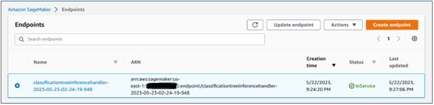
You can also check the training job status from the SageMaker console:

After the training jobs finishes, selecting the job link takes you to the job description page where you can see the MATLAB model saved in the dedicated S3 bucket:

Part 5: Deploy the model as a real-time SageMaker endpoint
After training, you can deploy the model as a real-time SageMaker endpoint, which you can use to make predictions in real time. To do this, call the deploy method from the estimator. This is where you can set up the desired instance size for hosting depending on the workload.
Behind the scenes, this step builds an inference docker image and pushes it to the Amazon ECR repository, nothing is required from the user to build the inference container. The image contains all the necessary information to serve the inference request, such as model location, MATLAB authentication information, and algorithms. After that, Amazon SageMaker creates a SageMaker endpoint configuration and finally deploys the real-time endpoint. The endpoint can be monitored in the SageMaker console and can be terminated anytime if it’s no longer used.
Part 6: Test the endpoint
Now that the endpoint is up and running, you can test the endpoint by giving it a few records to predict. Use the following code to select 10 records from the training data and send them to the endpoint for prediction. The prediction result is sent back from the endpoint and shown in the following image.

Part 7: Dashboard integration
The SageMaker endpoint can be called by many native AWS services. It can also be used as a standard REST API if deployed together with an AWS Lambda function and API gateway, which can be integrated with any web applications. For this particular use case, you can use streaming ingestion with Amazon SageMaker Feature Store and Amazon Managed Streaming for Apache Kafka, MSK, to make machine learning-backed decisions in near real-time. Another possible integration is using a combination of Amazon Kinesis, SageMaker, and Apache Flink to build a managed, reliable, scalable, and highly available application that’s capable of real-time inferencing on a data stream.
After algorithms are deployed to a SageMaker endpoint, you might want to visualize them using a dashboard that displays streaming predictions in real time. In the custom MATLAB web app that follows, you can see pressure and flow data by pump, and live fault predictions from the deployed model.
In this dashboard includes a remaining useful life (RUL) model to predict the time to failure for each pump in question. To learn how to train RUL algorithms, see Predictive Maintenance Toolbox.

Clean Up
After you run this solution, make sure you clean up any unneeded AWS resources to avoid unexpected costs. You can clean up these resources using the SageMaker Python SDK or the AWS Management Console for the specific services used here (SageMaker, Amazon ECR, and Amazon S3). By deleting these resources, you prevent further charges for resources you’re no longer using.
Conclusion
We’ve demonstrated how you can bring MATLAB to SageMaker for a pump predictive maintenance use case with the entire machine learning lifecycle. SageMaker provides a fully managed environment for running machine learning workloads and deploying models with a great selection of compute instances serving various needs.
Disclaimer: The code used in this post is owned and maintained by MathWorks. Refer to the license terms in the GitHub repo. For any issues with the code or feature requests, please open a GitHub issue in the repository
References
About the Authors
 Brad Duncan is the product manager for machine learning capabilities in the Statistics and Machine Learning Toolbox at MathWorks. He works with customers to apply AI in new areas of engineering such as incorporating virtual sensors in engineered systems, building explainable machine learning models, and standardizing AI workflows using MATLAB and Simulink. Before coming to MathWorks he led teams for 3D simulation and optimization of vehicle aerodynamics, user experience for 3D simulation, and product management for simulation software. Brad is also a guest lecturer at Tufts University in the area of vehicle aerodynamics.
 Richard Alcock is the senior development manager for Cloud Platform Integrations at MathWorks. In this role, he is instrumental in seamlessly integrating MathWorks products into cloud and container platforms. He creates solutions that enable engineers and scientists to harness the full potential of MATLAB and Simulink in cloud-based environments. He was previously a software engineering at MathWorks, developing solutions to support parallel and distributed computing workflows.
 Rachel Johnson is the product manager for predictive maintenance at MathWorks, and is responsible for overall product strategy and marketing. She was previously an application engineer directly supporting the aerospace industry on predictive maintenance projects. Prior to MathWorks, Rachel was an aerodynamics and propulsion simulation engineer for the US Navy. She also spent several years teaching math, physics, and engineering.
 Shun Mao is a Senior AI/ML Partner Solutions Architect in the Emerging Technologies team at Amazon Web Services. He is passionate about working with enterprise customers and partners to design, deploy and scale AI/ML applications to derive their business values. Outside of work, he enjoys fishing, traveling and playing Ping-Pong.
 Ramesh Jatiya is a Solutions Architect in the Independent Software Vendor (ISV) team at Amazon Web Services. He is passionate about working with ISV customers to design, deploy and scale their applications in cloud to derive their business values. He is also pursuing an MBA in Machine Learning and Business Analytics from Babson College, Boston. Outside of work, he enjoys running, playing tennis and cooking.
- SEO Powered Content & PR Distribution. Get Amplified Today.
- PlatoData.Network Vertical Generative Ai. Empower Yourself. Access Here.
- PlatoAiStream. Web3 Intelligence. Knowledge Amplified. Access Here.
- PlatoESG. Carbon, CleanTech, Energy, Environment, Solar, Waste Management. Access Here.
- PlatoHealth. Biotech and Clinical Trials Intelligence. Access Here.
- Source: https://aws.amazon.com/blogs/machine-learning/machine-learning-with-matlab-and-amazon-sagemaker/