AutoML allows you to derive rapid, general insights from your data right at the beginning of a machine learning (ML) project lifecycle. Understanding up front which preprocessing techniques and algorithm types provide best results reduces the time to develop, train, and deploy the right model. It plays a crucial role in every model’s development process and allows data scientists to focus on the most promising ML techniques. Additionally, AutoML provides a baseline model performance that can serve as a reference point for the data science team.

An AutoML tool applies a combination of different algorithms and various preprocessing techniques to your data. For example, it can scale the data, perform univariate feature selection, conduct PCA at different variance threshold levels, and apply clustering. Such preprocessing techniques could be applied individually or be combined in a pipeline. Subsequently, an AutoML tool would train different model types, such as Linear Regression, Elastic-Net, or Random Forest, on different versions of your preprocessed dataset and perform hyperparameter optimization (HPO). Amazon SageMaker Autopilot eliminates the heavy lifting of building ML models. After providing the dataset, SageMaker Autopilot automatically explores different solutions to find the best model. But what if you want to deploy your tailored version of an AutoML workflow?

This post shows how to create a custom-made AutoML workflow on Amazon SageMaker using Amazon SageMaker Automatic Model Tuning with sample code available in a GitHub repo.

Solution overview

For this use case, let’s assume you are part of a data science team that develops models in a specialized domain. You have developed a set of custom preprocessing techniques and selected a number of algorithms that you typically expect to work well with your ML problem. When working on new ML use cases, you would like first to perform an AutoML run using your preprocessing techniques and algorithms to narrow down the scope of potential solutions.

For this example, you don’t use a specialized dataset; instead, you work with the California Housing dataset that you will import from Amazon Simple Storage Service (Amazon S3). The focus is to demonstrate the technical implementation of the solution using SageMaker HPO, which later can be applied to any dataset and domain.

The following diagram presents the overall solution workflow.

Prerequisites

The following are prerequisites for completing the walkthrough in this post:

Implement the solution

The full code is available in the GitHub repo.

The steps to implement the solution (as noted in the workflow diagram) are as follows:

1. Create a notebook instance and specify the following:
   1. For Notebook instance type, choose ml.t3.medium.
   2. For Elastic Inference, choose none.
   3. For Platform identifier, choose Amazon Linux 2, Jupyter Lab 3.
   4. For IAM role, choose the default AmazonSageMaker-ExecutionRole. If it doesn’t exist, create a new AWS Identity and Access Management (IAM) role and attach the AmazonSageMakerFullAccess IAM policy.

Note that you should create a minimally scoped execution role and policy in production.

2. Open the JupyterLab interface for your notebook instance and clone the GitHub repo.

You can do that by starting a new terminal session and running the git clone <REPO> command or by using the UI functionality, as shown in the following screenshot.

3. Open the automl.ipynb notebook file, select the conda_python3 kernel, and follow the instructions to trigger a set of HPO jobs.

To run the code without any changes, you need to increase the service quota for ml.m5.large for training job usage and Number of instances across all training jobs. AWS allows by default only 20 parallel SageMaker training jobs for both quotas. You need to request a quota increase to 30 for both. Both quota changes should typically be approved within a few minutes. Refer to Requesting a quota increase for more information.

If you don’t want to change the quota, you can simply modify the value of the MAX_PARALLEL_JOBS variable in the script (for example, to 5).

4. Each HPO job will complete a set of training job trials and indicate the model with optimal hyperparameters.
5. Analyze the results and deploy the best-performing model.

This solution will incur costs in your AWS account. The cost of this solution will depend on the number and duration of HPO training jobs. As these increase, so will the cost. You can reduce costs by limiting training time and configuring TuningJobCompletionCriteriaConfig according to the instructions discussed later in this post. For pricing information, refer to Amazon SageMaker Pricing.

In the following sections, we discuss the notebook in more detail with code examples and the steps to analyze the results and select the best model.

Initial setup

Let’s start with running the Imports & Setup section in the custom-automl.ipynb notebook. It installs and imports all the required dependencies, instantiates a SageMaker session and client, and sets the default Region and S3 bucket for storing data.

Data preparation

Download the California Housing dataset and prepare it by running the Download Data section of the notebook. The dataset is split into training and testing data frames and uploaded to the SageMaker session default S3 bucket.

The entire dataset has 20,640 records and 9 columns in total, including the target. The goal is to predict the median value of a house (medianHouseValue column). The following screenshot shows the top rows of the dataset.

Training script template

The AutoML workflow in this post is based on scikit-learn preprocessing pipelines and algorithms. The aim is to generate a large combination of different preprocessing pipelines and algorithms to find the best-performing setup. Let’s start with creating a generic training script, which is persisted locally on the notebook instance. In this script, there are two empty comment blocks: one for injecting hyperparameters and the other for the preprocessing-model pipeline object. They will be injected dynamically for each preprocessing model candidate. The purpose of having one generic script is to keep the implementation DRY (don’t repeat yourself).

#create base script
_script = """
import argparse
import joblib
import os
import numpy as np
import pandas as pd
from sklearn.metrics import mean_squared_error
from sklearn.pipeline import Pipeline, FeatureUnion
from sklearn.preprocessing import StandardScaler
from sklearn.decomposition import PCA
from sklearn.impute import SimpleImputer
from sklearn.cluster import KMeans
from sklearn.linear_model import ElasticNet
from sklearn.ensemble import RandomForestRegressor
from sklearn.ensemble import GradientBoostingRegressor
###########################
### Inference functions ###
###########################
def model_fn(model_dir):
clf = joblib.load(os.path.join(model_dir, "model.joblib"))
return clf
if __name__ == "__main__":
print("Extracting arguments")
parser = argparse.ArgumentParser()
# Hyperparameters
##### WILL BE INSERTED DYNAMICALLY #####
{}
############################
# Data, model, and output directories
parser.add_argument("--model-dir", type=str, default=os.environ.get("SM_MODEL_DIR"))
parser.add_argument("--train", type=str, default=os.environ.get("SM_CHANNEL_TRAIN"))
parser.add_argument("--test", type=str, default=os.environ.get("SM_CHANNEL_TEST"))
parser.add_argument("--train-file", type=str, default="train.parquet")
parser.add_argument("--test-file", type=str, default="test.parquet")
parser.add_argument("--features", type=str)
parser.add_argument("--target", type=str)
args, _ = parser.parse_known_args()
# Load and prepare data
train_df = pd.read_parquet(os.path.join(args.train, args.train_file))
test_df = pd.read_parquet(os.path.join(args.test, args.test_file))
X_train = train_df[args.features.split()]
X_test = test_df[args.features.split()]
y_train = train_df[args.target]
y_test = test_df[args.target]
# Train model
##### WILL BE INSERTED DYNAMICALLY #####
{}
{}
############################
pipeline = Pipeline([('preprocessor', preprocessor), ('model', model)])
pipeline.fit(X_train, y_train)
# Validate model and print metrics
rmse = mean_squared_error(y_test, pipeline.predict(X_test), squared=False)
print("RMSE: " + str(rmse))
# Persist model
path = os.path.join(args.model_dir, "model.joblib")
joblib.dump(pipeline, path) """
# write _script to file just to have it in hand
with open("script_draft.py", "w") as f:
print(_script, file=f)

Create preprocessing and model combinations

The preprocessors dictionary contains a specification of preprocessing techniques applied to all input features of the model. Each recipe is defined using a Pipeline or a FeatureUnion object from scikit-learn, which chains together individual data transformations and stack them together. For example, mean-imp-scale is a simple recipe that ensures that missing values are imputed using mean values of respective columns and that all features are scaled using the StandardScaler. In contrast, the mean-imp-scale-pca recipe chains together a few more operations:

1. Impute missing values in columns with its mean.
2. Apply feature scaling using mean and standard deviation.
3. Calculate PCA on top of the input data at a specified variance threshold value and merge it together with the imputed and scaled input features.

In this post, all input features are numeric. If you have more data types in your input dataset, you should specify a more complicated pipeline where different preprocessing branches are applied to different feature type sets.

preprocessors = { "mean-imp-scale": "preprocessor = Pipeline([('imputer', SimpleImputer(strategy='mean')), ('scaler', StandardScaler())])n", "mean-imp-scale-knn": "preprocessor = FeatureUnion([('base-features', Pipeline([('imputer', SimpleImputer(strategy='mean')), ('scaler', StandardScaler())])), ('knn', Pipeline([('imputer', SimpleImputer(strategy='mean')), ('scaler', StandardScaler()), ('knn', KMeans(n_clusters=10))]))])n", "mean-imp-scale-pca": "preprocessor = FeatureUnion([('base-features', Pipeline([('imputer', SimpleImputer(strategy='mean')), ('scaler', StandardScaler())])), ('pca', Pipeline([('imputer', SimpleImputer(strategy='mean')), ('scaler', StandardScaler()), ('pca', PCA(n_components=0.9))]))])n" }

The models dictionary contains specifications of different algorithms that you fit the dataset to. Every model type comes with the following specification in the dictionary:

• script_output – Points to the location of the training script used by the estimator. This field is filled dynamically when the models dictionary is combined with the preprocessors dictionary.
• insertions – Defines code that will be inserted into the script_draft.py and subsequently saved under script_output. The key “preprocessor” is intentionally left blank because this location is filled with one of the preprocessors in order to create multiple model-preprocessor combinations.
• hyperparameters – A set of hyperparameters that are optimized by the HPO job.
• include_cls_metadata – More configuration details required by the SageMaker Tuner class.

A full example of the models dictionary is available in the GitHub repository.

models = { "rf": { "script_output": None, "insertions": { # Arguments "arguments" : "parser.add_argument('--n_estimators', type=int, default=100)n"+ " parser.add_argument('--max_depth', type=int, default=None)n"+ " parser.add_argument('--min_samples_leaf', type=int, default=1)n"+ " parser.add_argument('--min_samples_split', type=int, default=2)n"+ " parser.add_argument('--max_features', type=str, default='auto')n", # Model call "preprocessor": None, "model_call" : "model = RandomForestRegressor(n_estimators=args.n_estimators,max_depth=args.max_depth,min_samples_leaf=args.min_samples_leaf,min_samples_split=args.min_samples_split,max_features=args.max_features)n" }, "hyperparameters": { "n_estimators": IntegerParameter(100, 2000, "Linear"), "max_depth": IntegerParameter(1, 100, "Logarithmic"), "min_samples_leaf": IntegerParameter(1, 6, "Linear"), "min_samples_split": IntegerParameter(2, 20, "Linear"), "max_features": CategoricalParameter(["auto", "sqrt", "log2"]), }, "include_cls_metadata": False, }
}

Next, let’s iterate through the preprocessors and models dictionaries and create all possible combinations. For example, if your preprocessors dictionary contains 10 recipes and you have 5 model definitions in the models dictionary, the newly created pipelines dictionary contains 50 preprocessor-model pipelines that are evaluated during HPO. Note that individual pipeline scripts are not created yet at this point. The next code block (cell 9) of the Jupyter notebook iterates through all preprocessor-model objects in the pipelines dictionary, inserts all relevant code pieces, and persists a pipeline-specific version of the script locally in the notebook. Those scripts are used in the next steps when creating individual estimators that you plug into the HPO job.

pipelines = {}
for model_name, model_spec in models.items(): pipelines[model_name] = {} for preprocessor_name, preprocessor_spec in preprocessors.items(): pipeline_name = f"{model_name}-{preprocessor_name}" pipelines[model_name][pipeline_name] = {} pipelines[model_name][pipeline_name]["insertions"] = {} pipelines[model_name][pipeline_name]["insertions"]["preprocessor"] = preprocessor_spec pipelines[model_name][pipeline_name]["hyperparameters"] = model_spec["hyperparameters"] pipelines[model_name][pipeline_name]["include_cls_metadata"] = model_spec["include_cls_metadata"] pipelines[model_name][pipeline_name]["insertions"]["arguments"] = model_spec["insertions"]["arguments"] pipelines[model_name][pipeline_name]["insertions"]["model_call"] = model_spec["insertions"]["model_call"] pipelines[model_name][pipeline_name]["script_output"] = f"scripts/{model_name}/script-{pipeline_name}.py"

Define estimators

You can now work on defining SageMaker Estimators that the HPO job uses after scripts are ready. Let’s start with creating a wrapper class that defines some common properties for all estimators. It inherits from the SKLearn class and specifies the role, instance count, and type, as well as which columns are used by the script as features and the target.

class SKLearnBase(SKLearn): def __init__( self, entry_point=".", # intentionally left blank, will be overwritten in the next function framework_version="1.2-1", role=sm_role, instance_count=1, instance_type="ml.c5.xlarge", hyperparameters={ "features": "medianIncome housingMedianAge totalRooms totalBedrooms population households latitude longitude", "target": "medianHouseValue", }, **kwargs, ): super(SKLearnBase, self).__init__( entry_point=entry_point, framework_version=framework_version, role=role, instance_count=instance_count, instance_type=instance_type, hyperparameters=hyperparameters, **kwargs )

Let’s build the estimators dictionary by iterating through all scripts generated before and located in the scripts directory. You instantiate a new estimator using the SKLearnBase class, with a unique estimator name, and one of the scripts. Note that the estimators dictionary has two levels: the top level defines a pipeline_family. This is a logical grouping based on the type of models to evaluate and is equal to the length of the models dictionary. The second level contains individual preprocessor types combined with the given pipeline_family. This logical grouping is required when creating the HPO job.

estimators = {}
for pipeline_family in pipelines.keys(): estimators[pipeline_family] = {} scripts = os.listdir(f"scripts/{pipeline_family}") for script in scripts: if script.endswith(".py"): estimator_name = script.split(".")[0].replace("_", "-").replace("script", "estimator") estimators[pipeline_family][estimator_name] = SKLearnBase( entry_point=f"scripts/{pipeline_family}/{script}", base_job_name=estimator_name, )

Define HPO tuner arguments

To optimize passing arguments into the HPO Tuner class, the HyperparameterTunerArgs data class is initialized with arguments required by the HPO class. It comes with a set of functions, which ensure HPO arguments are returned in a format expected when deploying multiple model definitions at once.

@dataclass
class HyperparameterTunerArgs: base_job_names: list[str] estimators: list[object] inputs: dict[str] objective_metric_name: str hyperparameter_ranges: list[dict] metric_definition: dict[str] include_cls_metadata: list[bool] def get_estimator_dict(self) -> dict: return {k:v for (k, v) in zip(self.base_job_names, self.estimators)} def get_inputs_dict(self) -> dict: return {k:v for (k, v) in zip(self.base_job_names, [self.inputs]*len(self.base_job_names))} def get_objective_metric_name_dict(self) -> dict: return {k:v for (k, v) in zip(self.base_job_names, [self.objective_metric_name]*len(self.base_job_names))} def get_hyperparameter_ranges_dict(self) -> dict: return {k:v for (k, v) in zip(self.base_job_names, self.hyperparameter_ranges)} def get_metric_definition_dict(self) -> dict: return {k:[v] for (k, v) in zip(self.base_job_names, [self.metric_definition]*len(self.base_job_names))} def get_include_cls_metadata_dict(self) -> dict: return {k:v for (k, v) in zip(self.base_job_names, self.include_cls_metadata)}

The next code block uses the previously introduced HyperparameterTunerArgs data class. You create another dictionary called hp_args and generate a set of input parameters specific to each estimator_family from the estimators dictionary. These arguments are used in the next step when initializing HPO jobs for each model family.

hp_args = {}
for estimator_family, estimators in estimators.items(): hp_args[estimator_family] = HyperparameterTunerArgs( base_job_names=list(estimators.keys()), estimators=list(estimators.values()), inputs={"train": s3_data_train.uri, "test": s3_data_test.uri}, objective_metric_name="RMSE", hyperparameter_ranges=[pipeline.get("hyperparameters") for pipeline in pipelines[estimator_family].values()], metric_definition={"Name": "RMSE", "Regex": "RMSE: ([0-9.]+).*$"}, include_cls_metadata=[pipeline.get("include_cls_metadata") for pipeline in pipelines[estimator_family].values()], )

Create HPO tuner objects

In this step, you create individual tuners for every estimator_family. Why do you create three separate HPO jobs instead of launching just one across all estimators? The HyperparameterTuner class is restricted to 10 model definitions attached to it. Therefore, each HPO is responsible for finding the best-performing preprocessor for a given model family and tuning that model family’s hyperparameters.

The following are a few more points regarding the setup:

• The optimization strategy is Bayesian, which means that the HPO actively monitors the performance of all trials and navigates the optimization towards more promising hyperparameter combinations. Early stopping should be set to Off or Auto when working with a Bayesian strategy, which handles that logic itself.
• Each HPO job runs for a maximum of 100 jobs and runs 10 jobs in parallel. If you’re dealing with larger datasets, you might want to increase the total number of jobs.
• Additionally, you may want to use settings that control how long a job runs and how many jobs your HPO is triggering. One way to do that is to set the maximum runtime in seconds (for this post, we set it to 1 hour). Another is to use the recently released TuningJobCompletionCriteriaConfig. It offers a set of settings that monitor the progress of your jobs and decide whether it is likely that more jobs will improve the result. In this post, we set the maximum number of training jobs not improving to 20. That way, if the score isn’t improving (for example, from the fortieth trial), you won’t have to pay for the remaining trials until max_jobs is reached.

STRATEGY = "Bayesian"
OBJECTIVE_TYPE = "Minimize"
MAX_JOBS = 100
MAX_PARALLEL_JOBS = 10
MAX_RUNTIME_IN_SECONDS = 3600
EARLY_STOPPING_TYPE = "Off"
# RANDOM_SEED = 42 # uncomment if you require reproducibility across runs
TUNING_JOB_COMPLETION_CRITERIA_CONFIG = TuningJobCompletionCriteriaConfig( max_number_of_training_jobs_not_improving=20, ) tuners = {}
for estimator_family, hp in hp_args.items(): tuners[estimator_family] = HyperparameterTuner.create( estimator_dict=hp.get_estimator_dict(), objective_metric_name_dict=hp.get_objective_metric_name_dict(), hyperparameter_ranges_dict=hp.get_hyperparameter_ranges_dict(), metric_definitions_dict=hp.get_metric_definition_dict(), strategy=STRATEGY, completion_criteria_config=TUNING_JOB_COMPLETION_CRITERIA_CONFIG, objective_type=OBJECTIVE_TYPE, max_jobs=MAX_JOBS, max_parallel_jobs=MAX_PARALLEL_JOBS, max_runtime_in_seconds=MAX_RUNTIME_IN_SECONDS, base_tuning_job_name=f"custom-automl-{estimator_family}", early_stopping_type=EARLY_STOPPING_TYPE, # early stopping of training jobs is not currently supported when multiple training job definitions are used # random_seed=RANDOM_SEED, )

Now let’s iterate through the tuners and hp_args dictionaries and trigger all HPO jobs in SageMaker. Note the usage of the wait argument set to False, which means that the kernel won’t wait until the results are complete and you can trigger all jobs at once.

It’s likely that not all training jobs will complete and some of them might be stopped by the HPO job. The reason for this is the TuningJobCompletionCriteriaConfig—the optimization finishes if any of the specified criteria is met. In this case, when the optimization criteria isn’t improving for 20 consecutive jobs.

for tuner, hpo in zip(tuners.values(), hp_args.values()): tuner.fit( inputs=hpo.get_inputs_dict(), include_cls_metadata=hpo.get_include_cls_metadata_dict(), wait=False, )

Analyze results

Cell 15 of the notebook checks if all HPO jobs are complete and combines all results in the form of a pandas data frame for further analysis. Before analyzing the results in detail, let’s take a high-level look at the SageMaker console.

At the top of the Hyperparameter tuning jobs page, you can see your three launched HPO jobs. All of them finished early and didn’t perform all 100 training jobs. In the following screenshot, you can see that the Elastic-Net model family completed the highest number of trials, whereas others didn’t need so many training jobs to find the best result.

You can open the HPO job to access more details, such as individual training jobs, job configuration, and the best training job’s information and performance.

Let’s produce a visualization based on the results to get more insights of the AutoML workflow performance across all model families.

From the following graph, you can conclude that the Elastic-Net model’s performance was oscillating between 70,000 and 80,000 RMSE and eventually stalled, as the algorithm wasn’t able to improve its performance despite trying various preprocessing techniques and hyperparameter values. It also seems that RandomForest performance varied a lot depending on the hyperparameter set explored by HPO, but despite many trials it couldn’t go below the 50,000 RMSE error. GradientBoosting achieved the best performance already from the start going below 50,000 RMSE. HPO tried to improve that result further but wasn’t able to achieve better performance across other hyperparameter combinations. A general conclusion for all HPO jobs is that not so many jobs were required to find the best performing set of hyperparameters for each algorithm. To further improve the result, you would need to experiment with creating more features and performing additional feature engineering.

You can also examine a more detailed view of the model-preprocessor combination to draw conclusions about the most promising combinations.

Select the best model and deploy it

The following code snippet selects the best model based on the lowest achieved objective value. You can then deploy the model as a SageMaker endpoint.

df_best_job = df_tuner_results.loc[df_tuner_results["FinalObjectiveValue"] == df_tuner_results["FinalObjectiveValue"].min()]
df_best_job
BEST_MODEL_FAMILY = df_best_job["TrainingJobFamily"].values[0] tuners.get(BEST_MODEL_FAMILY).best_training_job() tuners.get(BEST_MODEL_FAMILY).best_estimator() predictor = tuners.get(BEST_MODEL_FAMILY).deploy( initial_instance_count=1, instance_type="ml.c4.large", endpoint_name=f"custom-automl-endpoint-{BEST_MODEL_FAMILY}",
)

Clean up

To prevent unwanted charges to your AWS account, we recommend deleting the AWS resources that you used in this post:

1. On the Amazon S3 console, empty the data from the S3 bucket where the training data was stored.

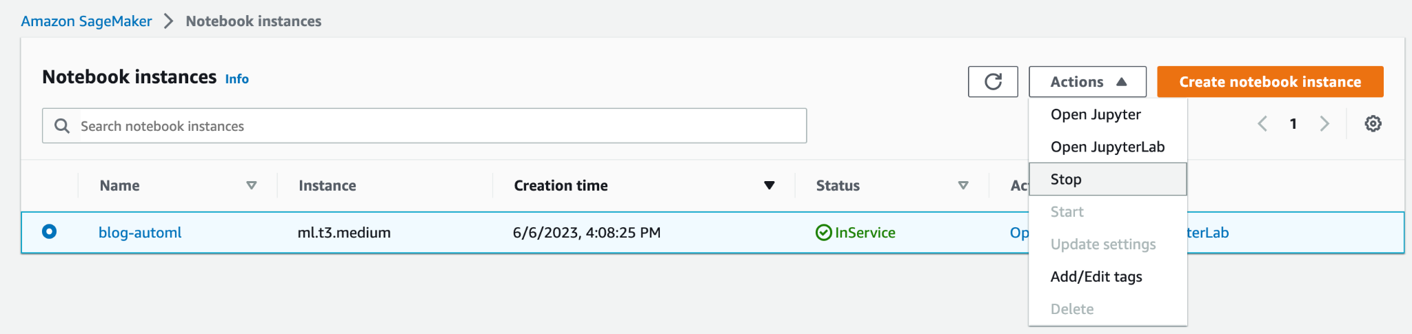
2. On the SageMaker console, stop the notebook instance.

3. Delete the model endpoint if you deployed it. Endpoints should be deleted when no longer in use, because they’re billed by time deployed.

sm_client.delete_endpoint(EndpointName=predictor.endpoint)

Conclusion

In this post, we showcased how to create a custom HPO job in SageMaker using a custom selection of algorithms and preprocessing techniques. In particular, this example demonstrates how to automate the process of generating many training scripts and how to use Python programming structures for efficient deployment of multiple parallel optimization jobs. We hope this solution will form the scaffolding of any custom model tuning jobs you will deploy using SageMaker to achieve higher performance and speed up of your ML workflows.

Check out the following resources to further deepen your knowledge of how to use SageMaker HPO:

About the Authors

Konrad Semsch is a Senior ML Solutions Architect at Amazon Web Services Data Lab Team. He helps customers use machine learning to solve their business challenges with AWS. He enjoys inventing and simplifying to enable customers with simple and pragmatic solutions for their AI/ML projects. He is most passionate about MlOps and traditional data science. Outside of work, he is a big fan of windsurfing and kitesurfing.

Tuna Ersoy is a Senior Solutions Architect at AWS. Her primary focus is helping Public Sector customers adopt cloud technologies for their workloads. She has a background in application development, enterprise architecture, and contact center technologies. Her interests include serverless architectures and AI/ML.

• SEO Powered Content & PR Distribution. Get Amplified Today.
• PlatoData.Network Vertical Generative Ai. Empower Yourself. Access Here.
• PlatoAiStream. Web3 Intelligence. Knowledge Amplified. Access Here.
• PlatoESG. Carbon, CleanTech, Energy, Environment, Solar, Waste Management. Access Here.
• PlatoHealth. Biotech and Clinical Trials Intelligence. Access Here.
• Source: https://aws.amazon.com/blogs/machine-learning/implement-a-custom-automl-job-using-pre-selected-algorithms-in-amazon-sagemaker-automatic-model-tuning/