Introduction

This guide is the second part of three guides about Support Vector Machines (SVMs). In this guide, we will keep working on the forged bank notes use case, understand what SVM parameters are already being set by Scikit-learn, what are C and Gamma hyperparameters, and how to tune them using cross validation and grid search.

In the complete series of SVM guides, besides SVM hyperparameters, you will also learn about simple SVM, a concept called the kernel trick, and explore other types of SVMs.

If you wish to read all the guides, take a look at the first guide, or see which ones interests you the most, below is the table of topics covered in each guide:

1. Implementing SVM and Kernel SVM with Python’s Scikit-Learn

• Use case: forget bank notes
• Background of SVMs
• Simple (Linear) SVM Model
  • About the Dataset
  • Importing the Dataset
  • Exploring the Dataset
• Implementing SVM with Scikit-Learn
  • Dividing Data into Train/Test Sets
  • Training the Model
  • Making Predictions
  • Evaluating the Model
  • Interpreting Results

2. Understanding SVM Hyperparameters

• The C Hyperparameter
• The Gamma Hyperparameter

3. Implementing other SVM flavors with Python’s Scikit-Learn (coming soon!)

• The General Idea of SVMs (a recap)
• Kernel (trick) SVM
• Implementing non-linear kernel SVM with Scikit-Learn
• Importing libraries
  • Importing the dataset
  • Dividing data into features (X) and target (y)
  • Dividing Data into Train/Test Sets
  • Training the Algorithm
• Polynomial kernel
  • Making Predictions
  • Evaluating the Algorithm
• Gaussian kernel
  • Prediction and Evaluation
• Sigmoid Kernel
  • Prediction and Evaluation
• Comparison of Non-Linear Kernel Performances

Let’s learn how to implement cross validation and perform a hyperparameter tuning.

SVM Hyperparameters

To see all model parameters that have already been set by Scikit-learn and its default values, we can use the get_params() method:

svc.get_params()

This method displays:

{'C': 1.0, 'break_ties': False, 'cache_size': 200, 'class_weight': None, 'coef0': 0.0, 'decision_function_shape': 'ovr', 'degree': 3, 'gamma': 'scale', 'kernel': 'linear', 'max_iter': -1, 'probability': False, 'random_state': None, 'shrinking': True, 'tol': 0.001, 'verbose': False}

Notice that there are a total of 15 hyperparameters already being set, this happens because the SVM algorithm has many variations. We have used the linear kernel to obtain a linear function, but there are also kernels that describe other kinds of functions and those kernels are parametrized in different ways.

These variations happen to make the model more flexible and suitable for finding a separation between different shapes of data. If we can draw a line to separate our classes, then a linear kernel will be a good option, if we need a curve, then a polynomial kernel might be the best choice, if our data has circular shapes, then a Radial Basis Function or RBF kernel will suit the data better, if there are values above and below a threshold, a sigmoid kernel might separate the classes better. From what we have explored in our data, it seems that either an RBF or a polynomial kernel would be more suitable than a linear kernel.

Now that we have an idea that there are 4 types of different kernel functions, we can go back to the parameters. When the SVM algorithm tries to find a separation between classes, we have already understood that it draws a classification margin between the support vectors and the separation line (or curve).

This margin is, in a sense, like a buffer between the separation line and the points. The margin size can vary, when the margin is smaller, there is less space for points that fall outside of the margin, making the separation between classes clearer, so more samples are being correctly classified, conversely, when the margin is larger, the separation between classes is less clear, and more samples can be misclassified. In other words, a smaller margin means more correctly classified samples, and also a more rigid classifier, while a larger margin, denotes more misclassified samples, but a more flexible classifier.

When those margins are chosen, the parameter that determines them is the C parameter.

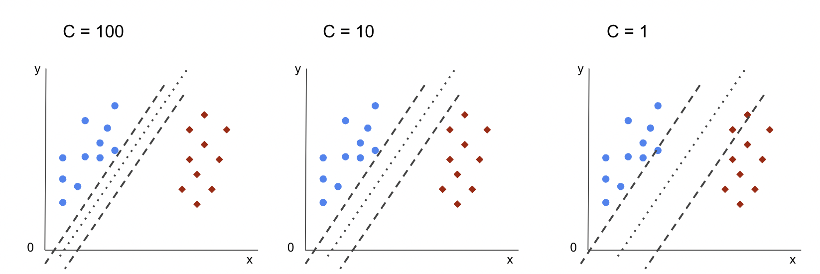
The C Hyperparameter

The C parameter is inversely proportional to the margin size, this means that the larger the value of C, the smaller the margin, and, conversely, the smaller the value of C, the larger the margin. The C parameter can be used along with any kernel, it tells the algorithm how much to avoid misclassifying each training sample, due to that, it is also known as regularization. Our linear kernel SVM has used a C of 1.0, which is a large value and gives a smaller margin.

We can experiment with a smaller value of ‘C’ and understand in practice what happens with a larger margin. To do that, we will create a new classifier, svc_c, and change only the value of C to 0.0001. Let’s also repeat the fit and predict steps:

svc_c = SVC(kernel='linear', C=0.0001)
svc_c.fit(X_train, y_train)
y_pred_c = svc_c.predict(X_test)

Now we can look at the results for the test data:

print(classification_report(y_test, y_pred_c)) cm_c = confusion_matrix(y_test, y_pred_c)
sns.heatmap(cm_c, annot=True, fmt='d').set_title('Confusion matrix of linear SVM with C=0.0001')

This outputs:

 precision recall f1-score support 0 0.82 0.96 0.88 148 1 0.94 0.76 0.84 127 accuracy 0.87 275 macro avg 0.88 0.86 0.86 275
weighted avg 0.88 0.87 0.86 275

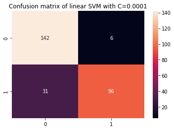
By using a smaller C and obtaining a larger margin, the classifier has become more flexible and with more classification mistakes. In the classification report, we can see that the f1-score, previously 0.99 for both classes, has lowered to 0.88 for class 0, and to 0.84 for class 1. In the confusion matrix, the model went from 2 to 6 false positives, and from 2 to 31 false negatives.

We can also repeat the predict step and look at the results to check if there is still an overfit when using train data:

y_pred_ct = svc_c.predict(X_train) cm_ct = confusion_matrix(y_train, y_pred_ct)
sns.heatmap(cm_ct, annot=True, fmt='d').set_title('Confusion matrix of linear SVM with C=0.0001 and train data') print(classification_report(y_train, y_pred_ct))

This results in:

 precision recall f1-score support 0 0.88 0.96 0.92 614 1 0.94 0.84 0.88 483 accuracy 0.90 1097 macro avg 0.91 0.90 0.90 1097
weighted avg 0.91 0.90 0.90 1097

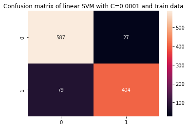
By looking at the results with a smaller C and train data, we can see there was an improvement in the overfit, but once most metrics are still higher for train data, it seems that the overfit hasn’t been solved. So, just changing the C parameter wasn’t enough to make the model more flexible and improve its generalization.

Up to this point, we have understood about the margins in SVM and how they impact the overall result of the algorithm, but how about the line (or curve) that separates the classes? This line is the decision boundary. So, we already know that the margins have an impact on the decision boundary flexibility towards mistakes, we can now take a look at another parameter that also impacts the decision boundary.

The Gamma Hyperparameter

Infinite decision boundaries can be chosen, some of those boundaries will separate the classes and others won’t. When choosing an effective decision boundary should the first 10 nearest points of each class be considered? Or should more points be considered, including the points that are far away? In SVM, that choice of range is defined by another hyperparameter, gamma.

Like C, gamma is somewhat inversely proportional to its distance. The higher its value, the closest are the points that are considered for the decision boundary, and the lowest the gamma, the farther points are also considered for choosing the decision boundary.

Another impact of gamma, is that the higher its value, the more the scope of the decision boundary gets closer to the points around it, making it more jagged and prone to overfit – and the lowest its value, the smoother and regular the decision boundary surface gets, also, less prone to overfit. This is true for any hyperplane, but can be easier observed when separating data in higher dimensions. In some documentations, gamma can also be referred to as sigma.

In the case of our model, the default value of gamma was scale. As it can be seen in the Scikit-learn SVC documentation, it means that its value is:

$$
gamma = (1/ text{n_features} * X.var())
$$

or

$$
gamma = (1/ text{number_of_features} * text{features_variance})
$$

In our case, we need to calculate the variance of X_train, multiply it by 4 and divide the result by 1. We can do this with the following code:

number_of_features = X_train.shape[1] features_variance = X_train.values.var()
gamma = 1/(number_of_features * features_variance)
print('gamma:', gamma)

This outputs:

gamma: 0.013924748072859962

There is also another way to look at the value of gamma, by accessing the classifier’s object gamma parameter with ._gamma:

svc._gamma 

We can see that the gamma used in our classifier was low, so it also considered farther away points.

There is no rule on how to choose values for hyperparameters, such as C and gamma – it will depend on how long and what resources are available for experimenting with different hyperparameter values, what transformations can be made to the data, and what results are expected. The usual way to search for the hyperparameter values is by combining each of the proposed values through a grid search along with a procedure that applies those hyperparameter values and obtains metrics for different parts of the data called cross validation. In Scikit-learn, this is already implemented as the GridSearchCV (CV from cross validation) method.

To run a grid search with cross validation, we need to import the GridSearchCV, define a dictionary with the values of hyperparameters that will be experimented with, such as the type of kernel, the range for C, and for gamma, create an instance of the SVC, define the score or metric will be used for evaluating (here we will chose to optimize for both precision and recall, so we’ll use f1-score), the number of divisions that will be made in the data for running the search in cv – the default is 5, but it is a good practice to use at least 10 – here, we will use 5 data folds to make it clearer when comparing results.

The GridSearchCV has a fit method that receives our train data and further splits it in train and test sets for the cross validation. We can set return_train_score to true to compare the results and guarantee there is no overfit.

This is the code for the grid search with cross validation:

from sklearn.model_selection import GridSearchCV parameters_dictionary = {'kernel':['linear', 'rbf'], 'C':[0.0001, 1, 10], 'gamma':[1, 10, 100]}
svc = SVC() grid_search = GridSearchCV(svc, parameters_dictionary, scoring = 'f1', return_train_score=True, cv = 5, verbose = 1) grid_search.fit(X_train, y_train)

This code outputs:

Fitting 5 folds for each of 18 candidates, totalling 90 fits
# and a clickable GridSeachCV object schema

After doing the hyperparameter search, we can use the best_estimator_, best_params_ and best_score_ properties to obtain the best model, parameter values and highest f1-score:

best_model = grid_search.best_estimator_
best_parameters = grid_search.best_params_
best_f1 = grid_search.best_score_ print('The best model was:', best_model)
print('The best parameter values were:', best_parameters)
print('The best f1-score was:', best_f1)

This results in:

The best model was: SVC(C=1, gamma=1)
The best parameter values were: {'C': 1, 'gamma': 1, 'kernel': 'rbf'}
The best f1-score was: 0.9979166666666666

Confirming our initial guess from looking at the data, the best model doesn’t have a linear kernel, but a nonlinear one, RBF.

Both C and gamma have the value of 1, and the f1-score is very high, 0.99. Since the value is high, let’s see if there was an overfit by peeking at the mean test and train scores we have returned, inside the cv_results_ object:

gs_mean_test_scores = grid_search.cv_results_['mean_test_score']
gs_mean_train_scores = grid_search.cv_results_['mean_train_score'] print("The mean test f1-scores were:", gs_mean_test_scores)
print("The mean train f1-scores were:", gs_mean_train_scores)

The mean scores were:

The mean test f1-scores were: [0.78017291 0. 0.78017291 0. 0.78017291 0. 0.98865407 0.99791667 0.98865407 0.76553515 0.98865407 0.040291 0.98656 0.99791667 0.98656 0.79182565 0.98656 0.09443985] The mean train f1-scores were: [0.78443424 0. 0.78443424 0. 0.78443424 0. 0.98762683 1. 0.98762683 1. 0.98762683 1. 0.98942923 1. 0.98942923 1. 0.98942923 1. ]

By looking at the mean scores, we can see that the highest one, 0.99791667 appears twice, and in both cases, the score in train data was 1. This indicates the overfit persists. From here, it would be interesting to go back to the data preparation and understand if it makes sense to normalize the data, make some other type of data transformation, and also create new features with feature engineering.

We have just seen a technique to find the model hyperparameters, and we have already mentioned something about linear separability, support vectors, decision boundary, maximization of margins, and kernel trick. SVM is a complex algorithm, usually with a lot of mathematical concepts involved and small tweakable parts that need to be adjusted to come together as a whole.

Let’s combine what we have seen so far, make a recap on how all the parts of SVM work, and then take a look at some of the other kernel implementations along with their results.

Conclusion

In this article we understood about the default parameters behind Scikit-Learn’s SVM implementation. We understood what C and Gamma parameters are, and how changing each one of them can impact the SVM model.

We also learned about grid search to look for the best C and Gamma values, and to use cross validation to better generalize our results and guarantee that there isn’t some form of data leakage.

Performing a hyperparameter tuning with grid search and cross validation is a common practice in data science, so I strongly suggest you implement the techniques, run the code and see the links between the hyperparameter values and the changes in SVM predictions.

• SEO Powered Content & PR Distribution. Get Amplified Today.
• Platoblockchain. Web3 Metaverse Intelligence. Knowledge Amplified. Access Here.
• Minting the Future w Adryenn Ashley. Access Here.
• Source: https://stackabuse.com/understanding-svm-hyperparameters/