Amazon SageMaker multi-model endpoints (MMEs) are a fully managed capability of SageMaker inference that allows you to deploy thousands of models on a single endpoint. Previously, MMEs pre-determinedly allocated CPU computing power to models statically regardless the model traffic load, using Multi Model Server (MMS) as its model server. In this post, we discuss a solution in which an MME can dynamically adjust the compute power assigned to each model based on the model’s traffic pattern. This solution enables you to use the underlying compute of MMEs more efficiently and save costs.

MMEs dynamically load and unload models based on incoming traffic to the endpoint. When utilizing MMS as the model server, MMEs allocate a fixed number of model workers for each model. For more information, refer to Model hosting patterns in Amazon SageMaker, Part 3: Run and optimize multi-model inference with Amazon SageMaker multi-model endpoints.

However, this can lead to a few issues when your traffic pattern is variable. Let’s say you have a singular or few models receiving a large amount of traffic. You can configure MMS to allocate a high number of workers for these models, but this gets assigned to all the models behind the MME because it’s a static configuration. This leads to a large number of workers using hardware compute—even the idle models. The opposite problem can happen if you set a small value for the number of workers. The popular models won’t have enough workers at the model server level to properly allocate enough hardware behind the endpoint for these models. The main issue is that it’s difficult to remain traffic pattern agnostic if you can’t dynamically scale your workers at the model server level to allocate the necessary amount of compute.

The solution we discuss in this post uses DJLServing as the model server, which can help mitigate some of the issues that we discussed and enable per-model scaling and enable MMEs to be traffic pattern agnostic.

MME architecture

SageMaker MMEs enable you to deploy multiple models behind a single inference endpoint that may contain one or more instances. Each instance is designed to load and serve multiple models up to its memory and CPU/GPU capacity. With this architecture, a software as a service (SaaS) business can break the linearly increasing cost of hosting multiple models and achieve reuse of infrastructure consistent with the multi-tenancy model applied elsewhere in the application stack. The following diagram illustrates this architecture.

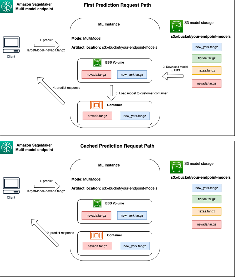
A SageMaker MME dynamically loads models from Amazon Simple Storage Service (Amazon S3) when invoked, instead of downloading all the models when the endpoint is first created. As a result, an initial invocation to a model might see higher inference latency than the subsequent inferences, which are completed with low latency. If the model is already loaded on the container when invoked, then the download step is skipped and the model returns the inferences with low latency. For example, assume you have a model that is only used a few times a day. It’s automatically loaded on demand, whereas frequently accessed models are retained in memory and invoked with consistently low latency.

Behind each MME are model hosting instances, as depicted in the following diagram. These instances load and evict multiple models to and from memory based on the traffic patterns to the models.

SageMaker continues to route inference requests for a model to the instance where the model is already loaded such that the requests are served from a cached model copy (see the following diagram, which shows the request path for the first prediction request vs. the cached prediction request path). However, if the model receives many invocation requests, and there are additional instances for the MME, SageMaker routes some requests to another instance to accommodate the increase. To take advantage of automated model scaling in SageMaker, make sure you have instance auto scaling set up to provision additional instance capacity. Set up your endpoint-level scaling policy with either custom parameters or invocations per minute (recommended) to add more instances to the endpoint fleet.

Model server overview

A model server is a software component that provides a runtime environment for deploying and serving machine learning (ML) models. It acts as an interface between the trained models and client applications that want to make predictions using those models.

The primary purpose of a model server is to allow effortless integration and efficient deployment of ML models into production systems. Instead of embedding the model directly into an application or a specific framework, the model server provides a centralized platform where multiple models can be deployed, managed, and served.

Model servers typically offer the following functionalities:

• Model loading – The server loads the trained ML models into memory, making them ready for serving predictions.
• Inference API – The server exposes an API that allows client applications to send input data and receive predictions from the deployed models.
• Scaling – Model servers are designed to handle concurrent requests from multiple clients. They provide mechanisms for parallel processing and managing resources efficiently to ensure high throughput and low latency.
• Integration with backend engines – Model servers have integrations with backend frameworks like DeepSpeed and FasterTransformer to partition large models and run highly optimized inference.

DJL architecture

DJL Serving is an open source, high performance, universal model server. DJL Serving is built on top of DJL, a deep learning library written in the Java programming language. It can take a deep learning model, several models, or workflows and make them available through an HTTP endpoint. DJL Serving supports deploying models from multiple frameworks like PyTorch, TensorFlow, Apache MXNet, ONNX, TensorRT, Hugging Face Transformers, DeepSpeed, FasterTransformer, and more.

DJL Serving offers many features that allow you to deploy your models with high performance:

• Ease of use – DJL Serving can serve most models out of the box. Just bring the model artifacts, and DJL Serving can host them.
• Multiple device and accelerator support – DJL Serving supports deploying models on CPU, GPU, and AWS Inferentia.
• Performance – DJL Serving runs multithreaded inference in a single JVM to boost throughput.
• Dynamic batching – DJL Serving supports dynamic batching to increase throughput.
• Auto scaling – DJL Serving will automatically scale workers up and down based on the traffic load.
• Multi-engine support – DJL Serving can simultaneously host models using different frameworks (such as PyTorch and TensorFlow).
• Ensemble and workflow models – DJL Serving supports deploying complex workflows comprised of multiple models, and runs parts of the workflow on CPU and parts on GPU. Models within a workflow can use different frameworks.

In particular, the auto scaling feature of DJL Serving makes it straightforward to ensure the models are scaled appropriately for the incoming traffic. By default, DJL Serving determines the maximum number of workers for a model that can be supported based on the hardware available (CPU cores, GPU devices). You can set lower and upper bounds for each model to make sure that a minimum traffic level can always be served, and that a single model doesn’t consume all available resources.

DJL Serving uses a Netty frontend on top of backend worker thread pools. The frontend uses a single Netty setup with multiple HttpRequestHandlers. Different request handlers will provide support for the Inference API, Management API, or other APIs available from various plugins.

The backend is based around the WorkLoadManager (WLM) module. The WLM takes care of multiple worker threads for each model along with the batching and request routing to them. When multiple models are served, WLM checks the inference request queue size of each model first. If the queue size is greater than two times a model’s batch size, WLM scales up the number of workers assigned to that model.

Solution overview

The implementation of DJL with an MME differs from the default MMS setup. For DJL Serving with an MME, we compress the following files in the model.tar.gz format that SageMaker Inference is expecting:

• model.joblib – For this implementation, we directly push the model metadata into the tarball. In this case, we are working with a .joblib file, so we provide that file in our tarball for our inference script to read. If the artifact is too large, you can also push it to Amazon S3 and point towards that in the serving configuration you define for DJL.
• serving.properties – Here you can configure any model server-related environment variables. The power of DJL here is that you can configure minWorkers and maxWorkers for each model tarball. This allows for each model to scale up and down at the model server level. For instance, if a singular model is receiving the majority of the traffic for an MME, the model server will scale the workers up dynamically. In this example, we don’t configure these variables and let DJL determine the necessary number of workers depending on our traffic pattern.
• model.py – This is the inference script for any custom preprocessing or postprocessing you would like to implement. The model.py expects your logic to be encapsulated in a handle method by default.
• requirements.txt (optional) – By default, DJL comes installed with PyTorch, but any additional dependencies you need can be pushed here.

For this example, we showcase the power of DJL with an MME by taking a sample SKLearn model. We run a training job with this model and then create 1,000 copies of this model artifact to back our MME. We then showcase how DJL can dynamically scale to handle any type of traffic pattern that your MME may receive. This can include an even distribution of traffic across all models or even a few popular models receiving the majority of the traffic. You can find all the code in the following GitHub repo.

Prerequisites

For this example, we use a SageMaker notebook instance with a conda_python3 kernel and ml.c5.xlarge instance. To perform the load tests, you can use an Amazon Elastic Compute Cloud (Amazon EC2) instance or a larger SageMaker notebook instance. In this example, we scale to over a thousand transactions per second (TPS), so we suggest testing on a heavier EC2 instance such as an ml.c5.18xlarge so that you have more compute to work with.

Create a model artifact

We first need to create our model artifact and data that we use in this example. For this case, we generate some artificial data with NumPy and train using an SKLearn linear regression model with the following code snippet:

import numpy as np
from sklearn.model_selection import train_test_split
from sklearn.linear_model import LinearRegression
import joblib

# Generate dummy data
np.random.seed(0)
X = np.random.rand(100, 1)
y = 2 * X + 1 + 0.1 * np.random.randn(100, 1)
# Split the data into training and testing sets
X_train, X_test, y_train, y_test = train_test_split(X, y, test_size=0.2, random_state=42)
# Create a Linear Regression model
model = LinearRegression()
# Train the model on the training data
model.fit(X_train, y_train)

# Create serialized model artifact
model_filename = "model.joblib"
joblib.dump(model, model_filename)

After you run the preceding code, you should have a model.joblib file created in your local environment.

Pull the DJL Docker image

The Docker image djl-inference:0.23.0-cpu-full-v1.0 is our DJL serving container used in this example. You can adjust the following URL depending on your Region:

inference_image_uri = "474422712127.dkr.ecr.us-east-1.amazonaws.com/djl-serving-cpu:latest"

Optionally, you can also use this image as a base image and extend it to build your own Docker image on Amazon Elastic Container Registry (Amazon ECR) with any other dependencies you need.

Create the model file

First, we create a file called serving.properties. This instructs DJLServing to use the Python engine. We also define the max_idle_time of a worker to be 600 seconds. This makes sure that we take longer to scale down the number of workers we have per model. We don’t adjust minWorkers and maxWorkers that we can define and we let DJL dynamically compute the number of workers needed depending on the traffic each model is receiving. The serving.properties is shown as follows. To see the complete list of configuration options, refer to Engine Configuration.

engine=Python
max_idle_time=600

Next, we create our model.py file, which defines the model loading and inference logic. For MMEs, each model.py file is specific to a model. Models are stored in their own paths under the model store (usually /opt/ml/model/). When loading models, they will be loaded under the model store path in their own directory. The full model.py example in this demo can be seen in the GitHub repo.

We create a model.tar.gz file that includes our model (model.joblib), model.py, and serving.properties:

#Build tar file with model data + inference code, replace this cell with your model.joblib
bashCommand = "tar -cvpzf model.tar.gz model.joblib requirements.txt model.py serving.properties"
process = subprocess.Popen(bashCommand.split(), stdout=subprocess.PIPE)
output, error = process.communicate()

For demonstration purposes, we make 1,000 copies of the same model.tar.gz file to represent the large number of models to be hosted. In production, you need to create a model.tar.gz file for each of your models.

Lastly, we upload these models to Amazon S3.

Create a SageMaker model

We now create a SageMaker model. We use the ECR image defined earlier and the model artifact from the previous step to create the SageMaker model. In the model setup, we configure Mode as MultiModel. This tells DJLServing that we’re creating an MME.

mme_model_name = "sklearn-djl-mme" + strftime("%Y-%m-%d-%H-%M-%S", gmtime())
print("Model name: " + mme_model_name)

create_model_response = sm_client.create_model(
ModelName=mme_model_name,
ExecutionRoleArn=role,
PrimaryContainer={"Image": inference_image_uri, "Mode": "MultiModel", "ModelDataUrl": mme_artifacts},
)

Create a SageMaker endpoint

In this demo, we use 20 ml.c5d.18xlarge instances to scale to a TPS in the thousands range. Make sure to get a limit increase on your instance type, if necessary, to achieve the TPS you are targeting.

mme_epc_name = "sklearn-djl-mme-epc" + strftime("%Y-%m-%d-%H-%M-%S", gmtime())
endpoint_config_response = sm_client.create_endpoint_config(
EndpointConfigName=mme_epc_name,
ProductionVariants=[
{
"VariantName": "sklearnvariant",
"ModelName": mme_model_name,
"InstanceType": "ml.c5d.18xlarge",
"InitialInstanceCount": 20
},],)

Load testing

At the time of writing, the SageMaker in-house load testing tool Amazon SageMaker Inference Recommender doesn’t natively support testing for MMEs. Therefore, we use the open source Python tool Locust. Locust is straightforward to set up and can track metrics such as TPS and end-to-end latency. For a full understanding of how to set it up with SageMaker, see Best practices for load testing Amazon SageMaker real-time inference endpoints.

In this use case, we have three different traffic patterns we want to simulate with MMEs, so we have the following three Python scripts that align with each pattern. Our goal here is to prove that, regardless of what our traffic pattern is, we can achieve the same target TPS and scale appropriately.

We can specify a weight in our Locust script to assign traffic across different portions of our models. For instance, with our single hot model, we implement two methods as follows:

# popular model
def sendPopular(self):

        request_meta = {
            "request_type": "InvokeEndpoint",
            "name": "SageMaker",
            "start_time": time.time(),
            "response_length": 0,
            "response": None,
            "context": {},
            "exception": None,
        }
        start_perf_counter = time.perf_counter()
        try:
            response = self.sagemaker_client.invoke_endpoint(
                EndpointName=self.endpoint_name,
                Body=self.payload,
                ContentType=self.content_type,
                TargetModel = "sklearn-0.tar.gz"
            )
  
# rest of model          
def sendRest(self):

        request_meta = {
            "request_type": "InvokeEndpoint",
            "name": "SageMaker",
            "start_time": time.time(),
            "response_length": 0,
            "response": None,
            "context": {},
            "exception": None,
        }
        start_perf_counter = time.perf_counter()
   
        try:
            response = self.sagemaker_client.invoke_endpoint(
                EndpointName=self.endpoint_name,
                Body=self.payload,
                ContentType=self.content_type,
                TargetModel = f'sklearn-{random.randint(1,989)}.tar.gz'
            )
            response_body = response["Body"].read()

We can then assign a certain weight to each method, which is when a certain method receives a specific percentage of the traffic:

# assign weights to models
class MyUser(BotoUser):

# 90% of traffic to singular model
@task(9)
def send_request(self):
self.client.sendPopular()

@task
def send_request_major(self):
self.client.sendRest()

For 20 ml.c5d.18xlarge instances, we see the following invocation metrics on the Amazon CloudWatch console. These values remain fairly consistent across all three traffic patterns. To understand CloudWatch metrics for SageMaker real-time inference and MMEs better, refer to SageMaker Endpoint Invocation Metrics.

You can find the rest of the Locust scripts in the locust-utils directory in the GitHub repository.

Summary

In this post, we discussed how an MME can dynamically adjust the compute power assigned to each model based on the model’s traffic pattern. This newly launched feature is available in all AWS Regions where SageMaker is available. Note that at the time of announcement, only CPU instances are supported. To learn more, refer to Supported algorithms, frameworks, and instances.

About the Authors

Ram Vegiraju is a ML Architect with the SageMaker Service team. He focuses on helping customers build and optimize their AI/ML solutions on Amazon SageMaker. In his spare time, he loves traveling and writing.

Qingwei Li is a Machine Learning Specialist at Amazon Web Services. He received his Ph.D. in Operations Research after he broke his advisor’s research grant account and failed to deliver the Nobel Prize he promised. Currently he helps customers in the financial service and insurance industry build machine learning solutions on AWS. In his spare time, he likes reading and teaching.

James Wu is a Senior AI/ML Specialist Solution Architect at AWS. helping customers design and build AI/ML solutions. James’s work covers a wide range of ML use cases, with a primary interest in computer vision, deep learning, and scaling ML across the enterprise. Prior to joining AWS, James was an architect, developer, and technology leader for over 10 years, including 6 years in engineering and 4 years in marketing & advertising industries.

Saurabh Trikande is a Senior Product Manager for Amazon SageMaker Inference. He is passionate about working with customers and is motivated by the goal of democratizing machine learning. He focuses on core challenges related to deploying complex ML applications, multi-tenant ML models, cost optimizations, and making deployment of deep learning models more accessible. In his spare time, Saurabh enjoys hiking, learning about innovative technologies, following TechCrunch and spending time with his family.

Xu Deng is a Software Engineer Manager with the SageMaker team. He focuses on helping customers build and optimize their AI/ML inference experience on Amazon SageMaker. In his spare time, he loves traveling and snowboarding.

Siddharth Venkatesan is a Software Engineer in AWS Deep Learning. He currently focusses on building solutions for large model inference. Prior to AWS he worked in the Amazon Grocery org building new payment features for customers world-wide. Outside of work, he enjoys skiing, the outdoors, and watching sports.

Rohith Nallamaddi is a Software Development Engineer at AWS. He works on optimizing deep learning workloads on GPUs, building high performance ML inference and serving solutions. Prior to this, he worked on building microservices based on AWS for Amazon F3 business. Outside of work he enjoys playing and watching sports.

• SEO Powered Content & PR Distribution. Get Amplified Today.
• PlatoData.Network Vertical Generative Ai. Empower Yourself. Access Here.
• PlatoAiStream. Web3 Intelligence. Knowledge Amplified. Access Here.
• PlatoESG. Carbon, CleanTech, Energy, Environment, Solar, Waste Management. Access Here.
• PlatoHealth. Biotech and Clinical Trials Intelligence. Access Here.
• Source: https://aws.amazon.com/blogs/machine-learning/run-ml-inference-on-unplanned-and-spiky-traffic-using-amazon-sagemaker-multi-model-endpoints/