In the world of data-driven decision-making, time series forecasting is key in enabling businesses to use historical data patterns to anticipate future outcomes. Whether you are working in asset risk management, trading, weather prediction, energy demand forecasting, vital sign monitoring, or traffic analysis, the ability to forecast accurately is crucial for success.
In these applications, time series data can have heavy-tailed distributions, where the tails represent extreme values. Accurate forecasting in these regions is important in determining how likely an extreme event is and whether to raise an alarm. However, these outliers significantly impact the estimation of the base distribution, making robust forecasting challenging. Financial institutions rely on robust models to predict outliers such as market crashes. In energy, weather, and healthcare sectors, accurate forecasts of infrequent but high-impact events such as natural disasters and pandemics enable effective planning and resource allocation. Neglecting tail behavior can lead to losses, missed opportunities, and compromised safety. Prioritizing accuracy at the tails helps lead to reliable and actionable forecasts. In this post, we train a robust time series forecasting model capable of capturing such extreme events using Amazon SageMaker.
To effectively train this model, we establish an MLOps infrastructure to streamline the model development process by automating data preprocessing, feature engineering, hyperparameter tuning, and model selection. This automation reduces human error, improves reproducibility, and accelerates the model development cycle. With a training pipeline, businesses can efficiently incorporate new data and adapt their models to evolving conditions, which helps ensure that forecasts remain reliable and up to date.
After the time series forecasting model is trained, deploying it within an endpoint grants real-time prediction capabilities. This empowers you to make well-informed and responsive decisions based on the most recent data. Furthermore, deploying the model in an endpoint enables scalability, because multiple users and applications can access and utilize the model simultaneously. By following these steps, businesses can harness the power of robust time series forecasting to make informed decisions and stay ahead in a rapidly changing environment.
Overview of solution
This solution showcases the training of a time series forecasting model, specifically designed to handle outliers and variability in data using a Temporal Convolutional Network (TCN) with a Spliced Binned Pareto (SBP) distribution. For more information about a multimodal version of this solution, refer to The science behind NFL Next Gen Stats’ new passing metric. To further illustrate the effectiveness of the SBP distribution, we compare it with the same TCN model but using a Gaussian distribution instead.
This process significantly benefits from the MLOps features of SageMaker, which streamline the data science workflow by harnessing the powerful cloud infrastructure of AWS. In our solution, we use Amazon SageMaker Automatic Model Tuning for hyperparameter search, Amazon SageMaker Experiments for managing experiments, Amazon SageMaker Model Registry to manage model versions, and Amazon SageMaker Pipelines to orchestrate the process. We then deploy our model to a SageMaker endpoint to obtain real-time predictions.
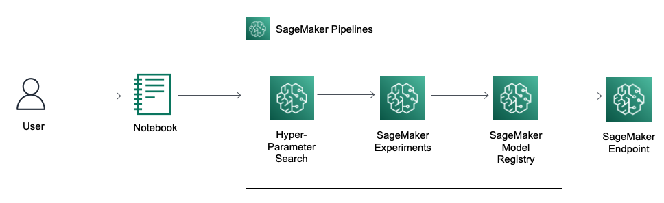
The following diagram illustrates the architecture of the training pipeline.
The following diagram illustrates the inference pipeline.

You can find the complete code in the GitHub repo. To implement the solution, run the cells in SBP_main.ipynb.
Click here to open the AWS console and follow along.
SageMaker pipeline
SageMaker Pipelines offers a user-friendly Python SDK to create integrated machine learning (ML) workflows. These workflows, represented as Directed Acyclic Graphs (DAGs), consist of steps with various types and dependencies. With SageMaker Pipelines, you can streamline the end-to-end process of training and evaluating models, enhancing efficiency and reproducibility in your ML workflows.
The training pipeline begins with generating a synthetic dataset that is split into training, validation, and test sets. The training set is used to train two TCN models, one utilizing Spliced Binned-Pareto distribution and the other employing Gaussian distribution. Both models go through hyperparameter tuning using the validation set to optimize each model. Afterward, an evaluation against the test set is conducted to determine the model with the lowest root mean squared error (RMSE). The model with the best accuracy metric is uploaded to the model registry.
The following diagram illustrates the pipeline steps.

Let’s discuss the steps in more detail.
Data generation
The first step in our pipeline generates a synthetic dataset, which is characterized by a sinusoidal waveform and asymmetric heavy-tailed noise. The data was created using a number of parameters, such as degrees of freedom, a noise multiplier, and a scale parameter. These elements influence the shape of the data distribution, modulate the random variability in our data, and adjust the spread of our data distribution, respectively.
This data processing job is accomplished using a PyTorchProcessor, which runs PyTorch code (generate_data.py) within a container managed by SageMaker. Data and other relevant artifacts for debugging are located in the default Amazon Simple Storage Service (Amazon S3) bucket associated with the SageMaker account. Logs for each step in the pipeline can be found in Amazon CloudWatch.
The following figure is a sample of the data generated by the pipeline.

You can replace the input with a wide variety of time series data, such as symmetric, asymmetric, light-tailed, heavy-tailed, or multimodal distribution. The model’s robustness allows it to be applicable to a broad range of time series problems, provided sufficient observations are available.
Model training
After data generation, we train two TCNs: one using SBP distribution and other using Gaussian distribution. SBP distribution employs a discrete binned distribution as its predictive base, where the real axis is divided into discrete bins, and the model predicts the likelihood of an observation falling within each bin. This methodology enables the capture of asymmetries and multiple modes because the probability of each bin is independent. An example of the binned distribution is shown in the following figure.
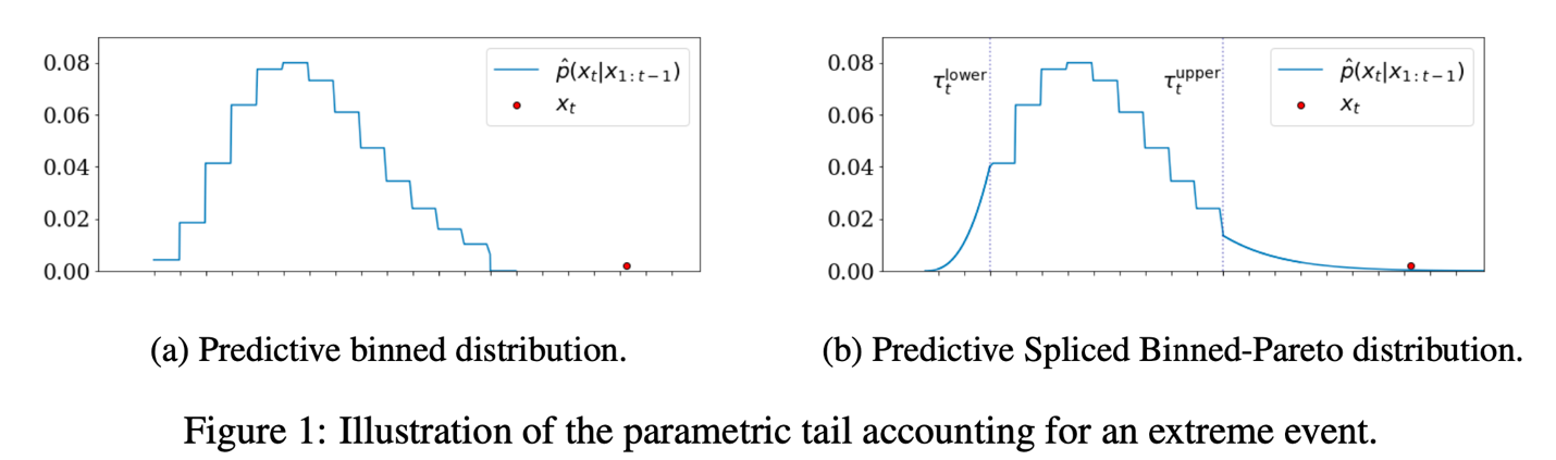
The predictive binned distribution on the left is robust to extreme events because the log-likelihood is not dependent on the distance between the predicted mean and observed point, differing from parametric distributions like Gaussian or Student’s t. Therefore, the extreme event represented by the red dot will not bias the learned mean of the distribution. However, the extreme event will have zero probability. To capture extreme events, we form an SBP distribution by defining the lower tail at the 5th quantile and the upper tail at the 95th quantile, replacing both tails with weighted Generalized Pareto Distributions (GPD), which can quantify the likeliness of the event. The TCN will output the parameters for the binned distribution base and GPD tails.
Hyperparameter search
For optimal output, we use automatic model tuning to find the best version of a model through hyperparameter tuning. This step is integrated into SageMaker Pipelines and allows for the parallel run of multiple training jobs, employing various methods and predefined hyperparameter ranges. The result is the selection of the best model based on the specified model metric, which is RMSE. In our pipeline, we specifically tune the learning rate and number of training epochs to optimize our model’s performance. With the hyperparameter tuning capability in SageMaker, we increase the likelihood that our model achieves optimal accuracy and generalization for the given task.
Due to the synthetic nature of our data, we are keeping Context Length and Lead Time as static parameters. Context Length refers to the number of historical time steps inputted into the model, and Lead Time represents the number of time steps in our forecast horizon. For the sample code, we are only tuning Learning Rate and the number of epochs to save on time and cost.
SBP-specific parameters are kept constant based on extensive testing by the authors on the original paper across different datasets:
- Number of Bins (100) – This parameter determines the number of bins used to model the base of the distribution. It is kept at 100, which has proven to be most effective across multiple industries.
- Percentile Tail (0.05) – This denotes the size of the generalized Pareto distributions at the tail. Like the previous parameter, this has been exhaustively tested and found to be most efficient.
Experiments
The hyperparameter process is integrated with SageMaker Experiments, which helps organize, analyze, and compare iterative ML experiments, providing insights and facilitating tracking of the best-performing models. Machine learning is an iterative process involving numerous experiments encompassing data variations, algorithm choices, and hyperparameter tuning. These experiments serve to incrementally refine model accuracy. However, the large number of training runs and model iterations can make it challenging to identify the best-performing models and make meaningful comparisons between current and past experiments. SageMaker Experiments addresses this by automatically tracking our hyperparameter tuning jobs and allowing us to gain further details and insight into the tuning process, as shown in the following screenshot.

Model evaluation
The models undergo training and hyperparameter tuning, and are subsequently evaluated via the evaluate.py script. This step utilizes the test set, distinct from the hyperparameter tuning stage, to gauge the model’s real-world accuracy. RMSE is used to assess the accuracy of the predictions.
For distribution comparison, we employ a probability-probability (P-P) plot, which assesses the fit between the actual vs. predicted distributions. The closeness of the points to the diagonal indicates a perfect fit. Our comparisons between SBP’s and Gaussian’s predicted distributions against the actual distribution show that SBP’s predictions align more closely with the actual data.
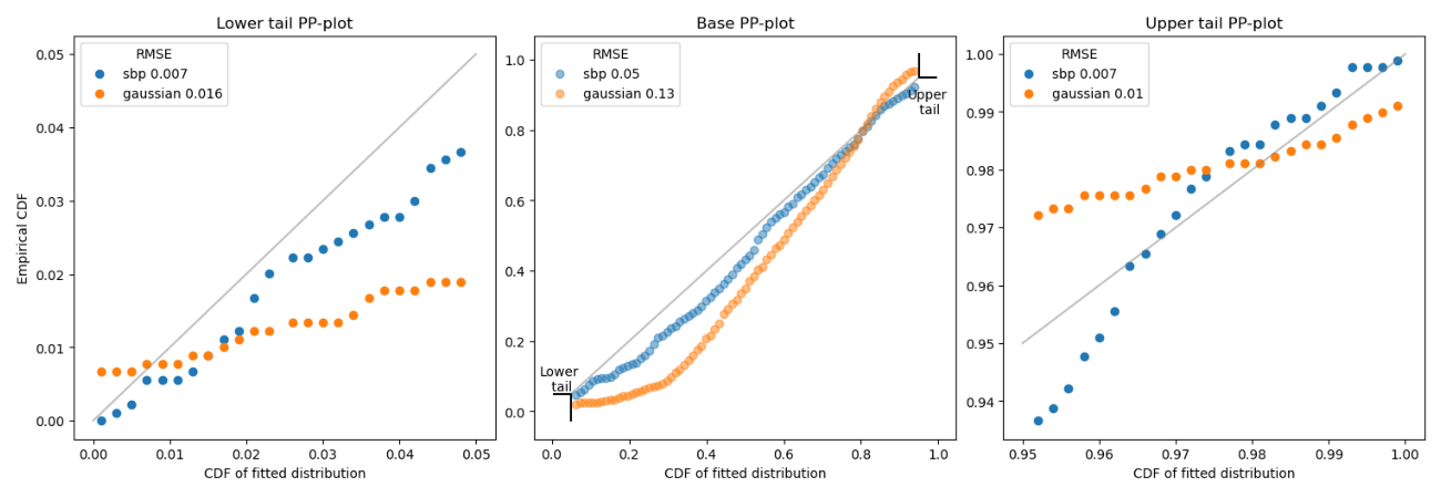
As we can observe, SBP has lower RMSE on the base, lower tail, and upper tail. The SBP distribution improved the accuracy of the Gaussian distribution by 61% on the base, 56% on the lower tail, and 30% on the upper tail. Overall, the SBP distribution has significantly better results.
Model selection
We use a condition step in SageMaker Pipelines to analyze model evaluation reports, opting for the model with the lowest RMSE for improved distribution accuracy. The selected model is converted into a SageMaker model object, readying it for deployment. This involves creating a model package with crucial parameters and packaging it into a ModelStep.
Model registry
The selected model is then uploaded to SageMaker Model Registry, which plays a critical role in managing models ready for production. It stores models, organizes model versions, captures essential metadata and artifacts such as container images, and governs the approval status of each model. By using the registry, we can efficiently deploy models to accessible SageMaker environments and establish a foundation for continuous integration and continuous deployment (CI/CD) pipelines.
Inference
Upon completion of our training pipeline, our model is then deployed using SageMaker hosting services, which enables the creation of an inference endpoint for real-time predictions. This endpoint allows seamless integration with applications and systems, providing on-demand access to the model’s predictive capabilities through a secure HTTPS interface. Real-time predictions can be used in scenarios such as stock price and energy demand forecast. Our endpoint provides a single-step forecast for the provided time series data, presented as percentiles and the median, as shown in the following figure and table.

| 1st percentile | 5th percentile | Median | 95th percentile | 99th percentile |
| 1.12 | 3.16 | 4.70 | 7.40 | 9.41 |
Clean up
After you run this solution, make sure you clean up any unnecessary AWS resources to avoid unexpected costs. You can clean up these resources using the SageMaker Python SDK, which can be found at the end of the notebook. By deleting these resources, you prevent further charges for resources you are no longer using.
Conclusion
Having an accurate forecast can highly impact a business’s future planning and can also provide solutions to a variety of problems in different industries. Our exploration of robust time series forecasting with MLOps on SageMaker has demonstrated a method to obtain an accurate forecast and the efficiency of a streamlined training pipeline.
Our model, powered by a Temporal Convolutional Network with Spliced Binned Pareto distribution, has shown accuracy and adaptability to outliers by improving the RMSE by 61% on the base, 56% on the lower tail, and 30% on the upper tail over the same TCN with Gaussian distribution. These figures make it a reliable solution for real-world forecasting needs.
The pipeline demonstrates the value of automating MLOps features. This can reduce manual human effort, enable reproducibility, and accelerate model deployment. SageMaker features such as SageMaker Pipelines, automatic model tuning, SageMaker Experiments, SageMaker Model Registry, and endpoints make this possible.
Our solution employs a miniature TCN, optimizing just a few hyperparameters with a limited number of layers, which are sufficient for effectively highlighting the model’s performance. For more complex use cases, consider using PyTorch or other PyTorch-based libraries to construct a more customized TCN that aligns with your specific needs. Additionally, it would be beneficial to explore other SageMaker features to enhance your pipeline’s functionality further. To fully automate the deployment process, you can use the AWS Cloud Development Kit (AWS CDK) or AWS CloudFormation.
For more information on time series forecasting on AWS, refer to the following:
Feel free to leave a comment with any thoughts or questions!
About the Authors
 Nick Biso is a Machine Learning Engineer at AWS Professional Services. He solves complex organizational and technical challenges using data science and engineering. In addition, he builds and deploys AI/ML models on the AWS Cloud. His passion extends to his proclivity for travel and diverse cultural experiences.
 Alston Chan is a Software Development Engineer at Amazon Ads. He builds machine learning pipelines and recommendation systems for product recommendations on the Detail Page. Outside of work, he enjoys game development and rock climbing.
 Maria Masood specializes in building data pipelines and data visualizations at AWS Commerce Platform. She has expertise in Machine Learning, covering natural language processing, computer vision, and time-series analysis. A sustainability enthusiast at heart, Maria enjoys gardening and playing with her dog during her downtime.
- SEO Powered Content & PR Distribution. Get Amplified Today.
- PlatoData.Network Vertical Generative Ai. Empower Yourself. Access Here.
- PlatoAiStream. Web3 Intelligence. Knowledge Amplified. Access Here.
- PlatoESG. Carbon, CleanTech, Energy, Environment, Solar, Waste Management. Access Here.
- PlatoHealth. Biotech and Clinical Trials Intelligence. Access Here.
- Source: https://aws.amazon.com/blogs/machine-learning/robust-time-series-forecasting-with-mlops-on-amazon-sagemaker/