This is a guest post co-authored by Ajay K Gupta, Jean Felipe Teotonio and Paul A Churchyard from HSR.health.

HSR.health is a geospatial health risk analytics firm whose vision is that global health challenges are solvable through human ingenuity and the focused and accurate application of data analytics. In this post, we present one approach for zoonotic disease prevention that uses Amazon SageMaker geospatial capabilities to create a tool that provides more accurate disease spread information to health scientists to help them save more lives, quicker.

Zoonotic diseases affect both animals and humans. The transition of a disease from animal to human, known as spillover, is a phenomenon that continually occurs on our planet. According to health organizations such as the Centers for Disease Control and Prevention (CDC) and the World Health Organization (WHO), a spillover event at a wet market in Wuhan, China most likely caused the coronavirus disease 2019 (COVID-19). Studies suggest that a virus found in fruit bats underwent significant mutations, allowing it to infect humans. The initial patient, or ‘patient zero’, for COVID-19 probably started a subsequent local outbreak that eventually spread on internationally. HSR.health’s Zoonotic Spillover Risk Index aims to assist in the identification of these early outbreaks before they cross international borders and lead to widespread global impact.

The main weapon public health has against the propagation of regional outbreaks is disease surveillance: an entire interlocking system of disease reporting, investigation, and data communication between different levels of a public health system. This system is dependent not only on human factors, but also on technology and resources to collect disease data, analyze patterns, and create a consistent and continuous stream of data transfer from local to regional to central health authorities.

The speed at which COVID-19 went from a local outbreak to a global disease present in every single continent should be a sobering example of the dire need to harness innovative technology to create more efficient and accurate disease surveillance systems.

The risk of zoonotic disease spillover is sharply correlated with multiple social, environmental, and geographic factors that influence how often human beings interact with wildlife. HSR.health’s Zoonotic Disease Spillover Risk Index uses over 20 distinct geographic, social, and environmental factors historically known to affect the risk of human-wildlife interaction and therefore zoonotic disease spillover risk. Many of these factors can be mapped through a combination of satellite imagery and remote sensing.

In this post, we explore how HSR.health uses SageMaker geospatial capabilities to retrieve relevant features from satellite imagery and remote sensing for developing the risk index. SageMaker geospatial capabilities make it easy for data scientists and machine learning (ML) engineers to build, train, and deploy models using geospatial data. With SageMaker geospatial capabilities, you can efficiently transform or enrich large-scale geospatial datasets, accelerate model building with pre-trained ML models, and explore model predictions and geospatial data on an interactive map using 3D accelerated graphics and built-in visualization tools.

Using ML and geospatial data for risk mitigation

ML is highly effective for anomaly detection on spatial or temporal data due to its ability to learn from data without being explicitly programmed to identify specific types of anomalies. Spatial data, which relates to the physical position and shape of objects, often contains complex patterns and relationships that may be difficult for traditional algorithms to analyze.

Incorporating ML with geospatial data enhances the capability to detect anomalies and unusual patterns systematically, which is essential for early warning systems. These systems are crucial in fields such as environmental monitoring, disaster management, and security. Predictive modeling using historical geospatial data allows organizations to identify and prepare for potential future events. These events range from natural disasters and traffic disruptions to, as this post discusses, disease outbreaks.

Detecting Zoonotic spillover risks

To predict zoonotic spillover risks, HSR.health has adopted a multimodal approach. By using a blend of data types—including environmental, biogeographical, and epidemiological information—this method enables a comprehensive assessment of disease dynamics. Such a multifaceted perspective is critical for developing proactive measures and enabling a rapid response to outbreaks.

The approach includes the following components:

• Disease and outbreak data – HSR.health uses the extensive disease and outbreak data provided by Gideon and the World Health Organization (WHO), two trusted sources of global epidemiological information. This data serves as a fundamental pillar in the analytics framework. For Gideon, the data can be accessed through an API, and for the WHO, HSR.health has built a large language model (LLM) to mine outbreak data from past disease outbreak reports.
• Earth observation data – Environmental factors, land use analysis and detection of habitat changes are integral components to assessing zoonotic risk. These insights can be derived from satellite-based earth observation data. HSR.health is able to streamline the use of earth observation data by using SageMaker geospatial capabilities to access and manipulate large-scale geospatial datasets. SageMaker geospatial offers a rich data catalog, including datasets from USGS Landsat-8, Sentinel-1, Sentinel-2, and others. It is also possible to bring in other datasets, such as high-resolution imagery from Planet Labs.
• Social determinants of risk – Beyond biological and environmental factors, the team at HSR.health also considered social determinants, which encompass various socioeconomic and demographic indicators, and play a pivotal role in shaping zoonotic spillover dynamics.

From these components, HSR.health evaluated a range of different factors, and the following features have been identified as influential for identifying zoonotic spillover risks:

• Animal habitats and habitable zones – Understanding the habitats of potential zoonotic hosts and their habitable zones is fundamental to assessing transmission risk.
• Population centers – Proximity to densely populated areas is a key consideration because it influences the likelihood of human-animal interactions.
• Loss of habitat – The degradation of natural habitats, particularly through deforestation, can accelerate zoonotic spillover events.
• Human-wildland interface – Areas where human settlements intersect with wildlife habitats are potential hotspots for zoonotic transmission.
• Social characteristics – Socioeconomic and cultural factors can significantly impact zoonotic risk, and HSR.health examines these as well.
• Human health characteristics – The health status of local human populations is an essential variable because it affects susceptibility and transmission dynamics.

Solution overview

HSR.health’s workflow encompasses data preprocessing, feature extraction, and the creation of informative visualizations using ML techniques. This allows for a clear understanding of the data’s evolution from its raw form to actionable insights.

The following is a visual representation of the workflow, starting with input data from Gideon, earth observation data, and social determinant of risk data.

Retrieve and process satellite imagery using SageMaker geospatial capabilities

Satellite data forms a cornerstone of the analysis performed to build the risk index, providing critical information on environmental changes. To generate insights from satellite imagery, HSR.health uses Earth Observation Jobs (EOJs). EOJs enable the acquisition and transformation of raster data gathered from the Earth’s surface. An EOJ obtains satellite imagery from a designated data source—for instance, a satellite constellation—over a specific area and time period. It then applies one or more models to the retrieved images.

Additionally, Amazon SageMaker Studio offers a geospatial notebook pre-installed with commonly-used geospatial libraries. This notebook enables direct visualization and processing of geospatial data within a Python notebook environment. EOJs can be created in the geospatial notebook environment.

To configure an EOJ, the following parameters are used:

• InputConfig – The input configuration specifies the data sources and the filtering criteria to be used during data acquisition:
  • RasterDataCollectionArn – Specifies the satellite from which to collect data.
  • AreaOfInterest – The geographical area of interest (AOI) defines the polygon boundaries for image collection.
  • TimeRangeFilter – The time range of interest: {StartTime: <string>, EndTime: <string>}.
  • PropertyFilters – Additional property filters, such as acceptable percentage of cloud coverage or desired sun azimuth angles.
• JobConfig – This configuration defines the type of job to be applied to the retrieved satellite image data. It supports operations such as band math, resampling, geomosaic or cloud removal.

The following example code demonstrates running an EOJ for cloud removal, representative of the steps performed by HSR.health:

eoj_input_config = { "RasterDataCollectionQuery": { "RasterDataCollectionArn": "arn:aws:sagemaker-geospatial:us-west-2:378778860802:raster-data-collection/public/nmqj48dcu3g7ayw8", "AreaOfInterest": { "AreaOfInterestGeometry": { "PolygonGeometry": { "Coordinates": [ [ [-76.23240119828894,-6.268815697653608], [-76.23240119828894,-6.339419992332921], [-76.13834453776985,-6.339419992332921], [-76.13834453776985,-6.268815697653608], [-76.23240119828894,-6.268815697653608] ] ] } } }, "TimeRangeFilter": { "StartTime": "2022-03-01T00:00:00Z", "EndTime": "2022-06-30T23:59:59Z", }, "PropertyFilters": { "Properties": [{"Property": {"EoCloudCover": {"LowerBound": 0.0, "UpperBound": 2.0}}}], "LogicalOperator": "AND", }, }
}
eoj_job_config = { "CloudRemovalConfig": { "AlgorithmName": "INTERPOLATION", "InterpolationValue": "-9999", "TargetBands": ["red", "green", "blue", "nir", "swir16"], }
} eoj = geospatial_client.start_earth_observation_job( Name="eoj-analysis-loreto", InputConfig=eoj_input_config, JobConfig=eoj_job_config, ExecutionRoleArn=execution_role,
)

HSR.health used several operations to preprocess the data and extract relevant features. This includes operations such as land cover classification, mapping temperature variation, and vegetation indexes.

One vegetation index relevant for indicating vegetation health is the Normalized Difference Vegetation Index (NDVI). The NDVI quantifies vegetation health by using near-infrared light, which vegetation reflects, and red light, which vegetation absorbs. Monitoring the NDVI over time can reveal changes in vegetation, such as the impact of human activities like deforestation.

The following code snippet demonstrates how to calculate a vegetation index like the NDVI based on the data that has been passed through cloud removal:

eoj_input_config = { "PreviousEarthObservationJobArn": eoj["Arn"]
}
eoj_job_config = { "BandMathConfig": { "CustomIndices": { "Operations": [ { "Equation": "(nir - red) / (nir + red)", "Name": "ndvi", "OutputType": "FLOAT32" } ] } }
}
eoj = geospatial_client.start_earth_observation_job( Name="eoj-vi-ndvi", InputConfig=eoj_input_config, JobConfig=eoj_job_config, ExecutionRoleArn=execution_role,
)

We can visualize the job output using SageMaker geospatial capabilities. SageMaker geospatial capabilities can help you overlay model predictions on a base map and provide layered visualization to make collaboration easier. With the GPU-powered interactive visualizer and Python notebooks, it’s possible to explore millions of data points in one view, facilitating the collaborative exploration of insights and results.

The steps outlined in this post demonstrate just one of the many raster-based features that HSR.health has extracted to create the risk index.

Combining raster-based features with health and social data

After extracting the relevant features in raster format, HSR.health used zonal statistics to aggregate the raster data within the administrative boundary polygons to which the social and health data are assigned. The analysis incorporates a combination of raster and vector geospatial data. This kind of aggregation allows for the management of raster data in a geodataframe, which facilitates its integration with the health and social data to produce the final risk index.

The following code snippet demonstrates how to aggregate raster data to administrative vector boundaries:

import geopandas as gp
import numpy as np
import pandas as pd
import rasterio
from rasterstats import zonal_stats
import pandas as pd def get_proportions(inRaster, inVector, classDict, idCols, year): # Reading In Vector File if '.parquet' in inVector: vector = gp.read_parquet(inVector) else: vector = gp.read_file(inVector) raster = rasterio.open(inRaster) vector = vector.to_crs(raster.crs) # Retrieving the Bounding Box for the Raster Image xmin, ymin, xmax, ymax = raster.bounds # Selecting the Vector Features that Intersect with the Raster Bounding Box vector = vector.cx[xmin:xmax, ymin:ymax] vector = vector.reset_index() # Calculate the sum of pixels of each class in the vector geometries stats = zonal_stats(vector.geometry, raster.read(1), affine=raster.transform, nodata=raster.nodata, categorical=True) # Creating a dataframe with the class sum of pixels and the id fields of the vector geometries df1 = pd.DataFrame(data=stats) df1 = df1.fillna(0) df1['totalpixels'] = df1.sum(axis=1) df1['year'] = year if 'year' in vector.columns.tolist(): vector = vector.drop(['year'], 1) # Merging the class sum of pixels dataframe with the vector geodataframe df = vector.merge(df1, left_index=True, right_index=True) # Renaming Columns cdict = pd.read_csv(classDict) cdict = cdict.set_index("Value")['Class_name'].to_dict() df = df.rename(columns=cdict) keptCols = [x for x in df.columns.tolist() if x in idCols + list(cdict.values()) + ['totalpixels', 'year']] df = df[keptCols] return(df) def aggregateData(rasterList, inVector, classDict, idCols, years): dfList = [] # Creating aggregated raster to vector geodataframes for all rasters in rasterList for tiff in rasterList: inRaster = tiff year = [x for x in years if x in tiff][0] dfList.append(get_proportions(inRaster, inVector, classDict, idCols, year)) # Concating into a single geodataframe allDf = pd.concat(dfList, ignore_index=True) classDictDf = pd.read_csv(classDict) # Renaming the numerical values of the categories to the string version of the category name classCols = classDictDf['Class_name'].unique().tolist() # Summing the pixel counts by administrative division as a single administrative division might cover more than one raster image for col in classCols: allDf[col] = allDf[col].fillna(0) allDf[col] = allDf.groupby(idCols + ['year'])[col].transform(lambda x: x.sum()) # Removing Duplicates from the dataframe allDf = allDf.groupby(idCols + ['year']).first().reset_index() # Reattaching the geometry to the aggregated raster data if '.parquet' in inVector: vector = gp.read_parquet(inVector) else: vector = gp.read_file(inVector) allDf = vector.merge(allDf, on=idCols) return(allDf)

To evaluate the extracted features effectively, ML models are used to predict factors representing each feature. One of the models used is a support vector machine (SVM). The SVM model assists in revealing patterns and associations within data that inform risk assessments.

The index represents a quantitative assessment of risk levels, calculated as a weighted average of these factors, to aid in understanding potential spillover events in various regions.

import pandas as pd
import numpy as np
import geopandas as gp def finalIndicatorCalculation(inputLayer, weightDictionary, outLayer): # Creating a dictionary with the weights for each factor in the indicator weightsDict = pd.read_csv(weightDictionary).set_index('metric')['weight'].to_dict() # Reading in the data from the layer layer = gp.read_file(inputLayer) # Initializing the Sum of the Weights layer['sumweight'] = 0 # Calculating the sum of the weighted factors for col in weightsDict.keys(): layer[col] = layer[col].fillna(0) layer['sumweight'] = layer['sumweight'] + (layer[col] * zweights[col]) # Calculating Raw Zoonotic Spillover Risk Index layer['raw_idx'] = np.log(layer['e_pop']) * layer['sumweight'] # Normalizing the Index between 0 and 100 layer['zs_idx'] = ((layer['raw_idx'] - layer['raw_idx'].min()) / (layer['raw_idx'].max() - layer['raw_idx'].min()) * 100).round(2) return(layer)

The following figure on the left shows the aggregation of the image classification from the test area scene in northern Peru aggregated to the district administrative level with the calculated change in the forest area between 2018–2023. Deforestation is one of the key factors that determine the risk of zoonotic spillover. The figure on the right highlights the zoonotic spillover risk severity levels within the regions covered, ranging from highest (red) to the lowest (dark green) risk. The area was chosen as one of the training areas for the image classification due to the diversity of land cover captured in the scene, including: urban, forest, sand, water, grassland, and agriculture, among others. Additionally, this is one of many areas of interest for potential zoonotic spillover events due to the deforestation and interaction between humans and animals.

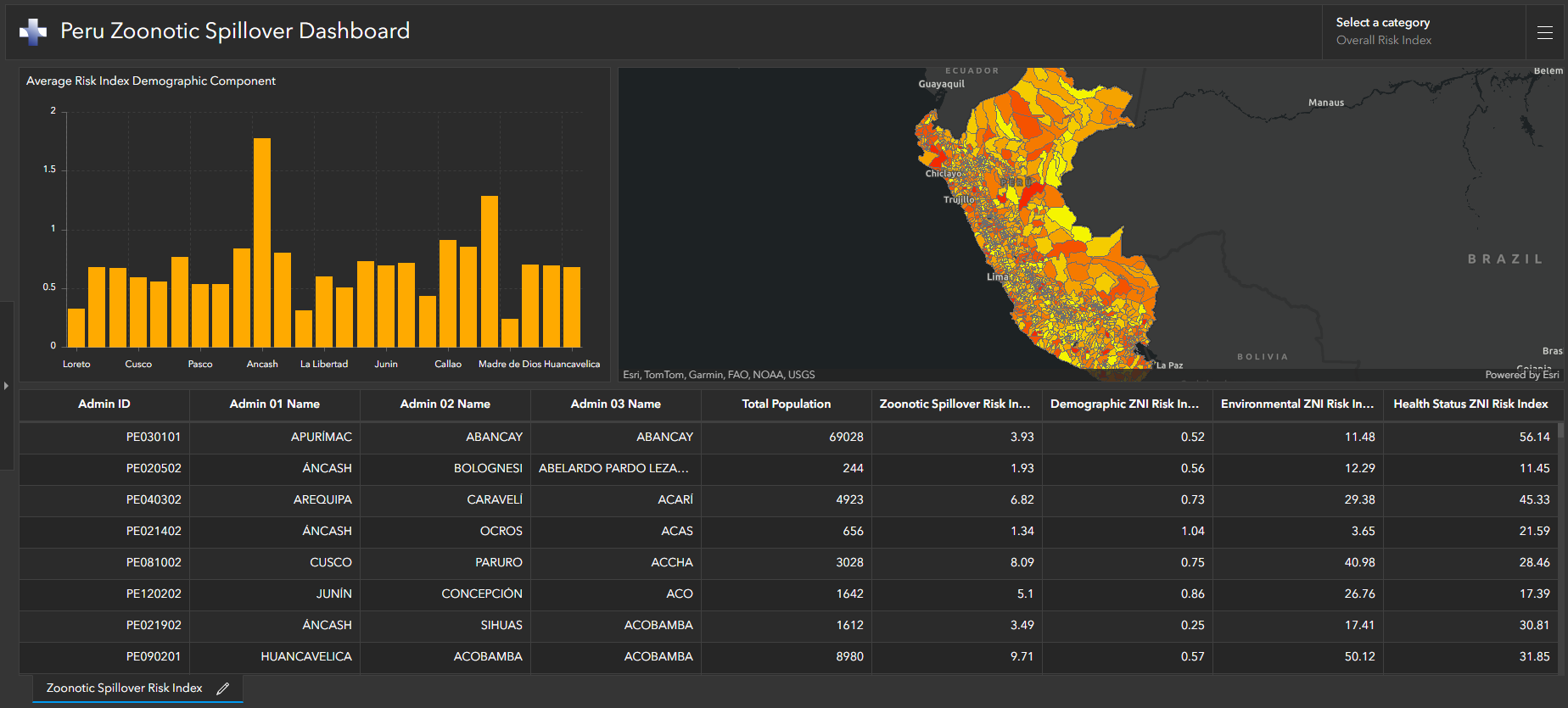
By adopting this multi-modal approach, encompassing historical data on disease outbreak, Earth observation data, social determinants, and ML techniques, we can better understand and predict zoonotic spillover risk, ultimately directing disease surveillance and prevention strategies to areas of greatest outbreak risk. The following screenshot shows a dashboard of the output from a zoonotic spillover risk analysis. This risk analysis highlights where resources and surveillance for new potential zoonotic outbreaks can occur so that the next disease can be contained before it becomes an endemic or a new pandemic.

A novel approach to pandemic prevention

In 1998, along the Nipah River in Malaysia, between the fall of 1998 and spring of 1999, 265 people were infected with a then unknown virus that caused acute encephalitis and severe respiratory distress. 105 of them died, a 39.6% fatality rate. COVID-19’s untreated fatality rate by contrast is 6.3%. Since then, the Nipah Virus, as it is now dubbed, has transitioned out of its forest habitat and caused over 20 deadly outbreaks, mostly in India and Bangladesh.

Viruses such as Nipah surface each year, posing challenges to our daily lives, particularly in countries where establishing strong, lasting, and robust systems for disease surveillance and detection is more difficult. These detection systems are crucial for reducing the risks associated with such viruses.

Solutions that use ML and geospatial data, such as the Zoonotic Spillover Risk Index, can assist local public health authorities in prioritizing resource allocation to areas of highest risk. By doing so, they can establish targeted and localized surveillance measures to detect and halt regional outbreaks before they extend beyond borders. This approach can significantly limit the impact of a disease outbreak and save lives.

Conclusion

This post demonstrated how HSR.health successfully developed the Zoonotic Spillover Risk Index by integrating geospatial data, health, social determinants, and ML. By using SageMaker, the team created a scalable workflow that can pinpoint the most substantial threats of a potential future pandemic. Effective management of these risks can lead to a reduction in the global disease burden. The substantial economic and social advantages of reducing pandemic risk cannot be overstated, with benefits extending regionally and globally.

HSR.health used SageMaker geospatial capabilities for an initial implementation of the Zoonotic Spillover Risk Index and is now seeking partnerships, as well as support from host countries and funding sources, to develop the index further and extend its application to additional regions around the world. For more information about HSR.health and the Zoonotic Spillover Risk Index, visit www.hsr.health.

Discover the potential of integrating Earth observation data into your healthcare initiatives by exploring SageMaker geospatial features. For more information, refer to Amazon SageMaker geospatial capabilities, or engage with additional examples to get hands-on experience.

About the Authors

Ajay K Gupta is Co-Founder and CEO of HSR.health, a firm that disrupts and innovates health risk analytics through geospatial tech and AI techniques to predict the spread and severity of disease. And provides these insights to industry, governments, and the health sector so they can anticipate, mitigate, and take advantage of future risks. Outside of work, you can find Ajay behind the mic bursting eardrums while belting out his favorite pop music tunes from U2, Sting, George Michael, or Imagine Dragons.

Jean Felipe Teotonio is a driven physician and passionate expert in healthcare quality and infectious disease epidemiology, Jean Felipe leads the HSR.health public health team. He works towards the shared goal of improving public health by reducing the global burden of disease by leveraging GeoAI approaches to develop solutions for the greatest health challenges of our time. Outside of work, his hobbies include reading sci fi books, hiking, the English premier league, and playing bass guitar.

Paul A Churchyard, CTO and Chief Geospatial Engineer for HSR.health, uses his broad technical skills and expertise to build the core infrastructure for the firm as well as its patented and proprietary GeoMD Platform. Additionally, he and the data science team incorporate geospatial analytics and AI/ML techniques into all health risk indices HSR.health produces. Outside of work, Paul is a self-taught DJ and loves snow.

Janosch Woschitz is a Senior Solutions Architect at AWS, specializing in geospatial AI/ML. With over 15 years of experience, he supports customers globally in leveraging AI and ML for innovative solutions that capitalize on geospatial data. His expertise spans machine learning, data engineering, and scalable distributed systems, augmented by a strong background in software engineering and industry expertise in complex domains such as autonomous driving.

Emmett Nelson is an Account Executive at AWS supporting Nonprofit Research customers across the Healthcare & Life Sciences, Earth / Environmental Sciences, and Education verticals. His primary focus is enabling use cases across analytics, AI/ML, high performance computing (HPC), genomics, and medical imaging. Emmett joined AWS in 2020 and is based in Austin, TX.

• SEO Powered Content & PR Distribution. Get Amplified Today.
• PlatoData.Network Vertical Generative Ai. Empower Yourself. Access Here.
• PlatoAiStream. Web3 Intelligence. Knowledge Amplified. Access Here.
• PlatoESG. Carbon, CleanTech, Energy, Environment, Solar, Waste Management. Access Here.
• PlatoHealth. Biotech and Clinical Trials Intelligence. Access Here.
• Source: https://aws.amazon.com/blogs/machine-learning/how-hsr-health-is-limiting-risks-of-disease-spillover-from-animals-to-humans-using-amazon-sagemaker-geospatial-capabilities/